Continuing with the theme of fast function approximations (see the previous post on Fresnel curve approximations), using my custom program search algorithm, I have come up with a fast approximate acos (arccosine) function.
Absolute error is <= 0.0004333.
The idea for the sqrt(2 - 2x) comes from Trey Reynolds
The reflectance of light hitting a dielectric (non-metal) / dielectric interface is something commonly needed in computer graphics, and one of the few material properties that we can get a compact and exact solution for, from Maxwell's equations.
In computer graphics, a faster approximation is often used - Schlick's approximation.
It kind of sucks tho - it has quite large relative error, resulting in visibly incorrect reflection.
For the n_1 = 1, n_2 = 1.5 case, the relative error is 23.2%, and for n_2=1.333, the relative error is 32.5% !
Schlick's approximation for n_2=1.3
Schlick's approximation for n_2=1.5
This has been bugging me for a while (a decade plus), so while fixing some NaNs I decided I should yak shave and look into it - can I do better?
It's hard to come up with a simple formula that can handle a range of IORs, but if you assume a fixed IOR, you can get some nice results.
These approximations are useful for applications like computer games, where all shaders may use a few fixed IOR values. For example your water shader will probably always have IOR 1.333.
It has relative and absolute error <= 0.00382. (0.3%)
As you can see, these approximations are much more accurate than Schlick's.
What's the performance like? These functions run in around 23 cycles on my Zen 3 CPU machine. This is significantly faster than the exact Fresnel reflectance code which runs in around 54 cycles.
I used a rational function (a ratio of two quadratic polynomials) as the approximating functions - I think rational functions are pretty cool - they can fit curves polynomials can't with very few parameters. I used a custom search program to find the coefficients.
I also did a program search for a formula that can approximate the Fresnel reflectance curve for a range of IORs, and found something - but it's not that much faster than the exact code, so not sure it's worth using.
camToScreenSpace takes something like 16 float multiplies and 12 additions for the matrix-vector mul, and 2 divides for the perspective divide.
So camSpaceDirToScreenSpaceDir takes something like 32 multiplies, 24 additions/subtractions, and 4 divides. That's quite a lot of operations!
We can do much better!
If you use the standard perspective projection with OpenGL camera-space (view-space) coordinate convention (+x to the right, +y up, +z out of screen back from camera), camToScreenSpace looks like
Where l is the sensor to lens distance, and w is the sensor width for a thin-lens perspective camera. \(l/w\) is also equal to \(2 \tan(\alpha)\) where \(\alpha\) is half the horizontal angle of view.
In maths:
$$ p_{ss_x} = {p_x \over -p_z} {l \over w} + {1 \over 2} \\
p_{ss_y} = {p_y \over -p_z} {l \over h} + {1 \over 2}
$$
Where \(p_{ss}\) is a point in screen space and \(p\) is a point in camera space.
So how can we get the screen-space direction from this?
Consider a ray in camera space, parameterised by t, such that a point along the ray at distance t is given by
$$
r(t) = p + t d
$$
Then the direction in screen space is given by
$$
{d \over dt} p_{ss} = ({d \over dt} p_{ss_x}, {d \over dt} p_{ss_y})
$$
Taking x coord first:
$$
{d \over dt} p_{ss_x} = {d \over dt} [ {p_x \over -p_z} {l \over w} + {1 \over 2} ]
$$
and substituting in our expression for the point on the ray \(p = r(t)\):
$$
{d \over dt} p_{ss_x} = {d \over dt} [ {r(t)_x \over -r(t)_z} {l \over w} + {1 \over 2} ]\\
= -{l \over w} {d \over dt} [ {r(t)_x \over r(t)_z}] \\
$$
Now we can use the quotient rule:
$$
{d \over dt} p_{ss_x} = -{l \over w} [ {{d \over dt} r(t)_x r(t)_z - r(t)_x {d \over dt} r(t)_z \over r(t)_z^2 } ]
$$
And substituting in our expressions for \(r(t)\):
$$
{d \over dt} p_{ss_x} = -{l \over w} [ {{d \over dt} (p_x + t d_x) (p_z + t d_z) - (p_x + t d_x) {d \over dt} (p_z + t d_z) \over (p_z + t d_z)^2 } ] \\
= -{l \over w} [ {d_x (p_z + t d_z) - (p_x + t d_x) d_z \over (p_z + t d_z)^2 } ] \\
= -{l \over w} [ {d_x p_z + t d_x d_z - p_x d_z - t d_x d_z \over (p_z + t d_z)^2 } ]\\
= -{l \over w} [ {d_x p_z - p_x d_z \over (p_z + t d_z)^2 } ]
$$
Evaluated at \(t=0\) gives
$$
{d \over dt} p_{ss_x} |_{t=0} = -{l \over w} [ {d_x p_z - p_x d_z \over p_z^2 } ]
$$
Likewise for the y coord:
$$
{d \over dt} p_{ss_y} |_{t=0} = -{l \over h} [ {d_y p_z - p_y d_z \over p_z^2 } ]
$$
If we are just interested in the unnormalised direction vector, we can drop the common \( {1\over p_z^2} \) factor, giving the vector result:
$$
d_{ss} = (-{l \over w} (d_x p_z - p_x d_z), -{l \over h} (d_y p_z - p_y d_z)) \\
= ({l \over w} (p_x d_z - d_x p_z), {l \over h} (p_y d_z - d_y p_z)) \\
$$
Or in code:
Writing the terrain generation and erosion simulation program TerrainGen requires computing how water flows downhill.
Among the forces acting on an element of water in a streambed are the viscous friction forces and the gravity force. The gravity force pulls the water downhill, and the viscous friction force slows the descent. Without viscous friction forces, water would 'flow' downhill kind of like a metal ball would roll down a surface - it would get faster and faster in a very unrealistic way.
So the viscous friction force is important for computing how to accelerate an element of water. But what is a good expression for this force? After browsing around a bit I found the Manning Formula, which gives the velocity of water flowing down a channel in terms of the channel slope etc. With a little bit of maths this can be turned into a force (or rather an acceleration):
The Manning Formula is
$$V = {k \over n} R_h^{2/3} S^{1/2} $$
Where \( V \) is the average velocity, \(n\) is the Gauckler–Manning coefficient, \(R_h\) is the hydraulic radius, \(S\) is the stream slope, and \(k\) is a conversion factor.
As the wikipedia article notes, for a wide rectangular channel, the hydraulic radius is approximated by the flow depth. So lets assume our channel is a wide rectangular channel with flow depth \(d\).
$$R_h \approx d$$
We will assume we have an infinitely long channel of constant slope \(\frac{\partial h}{\partial x}\) and constant cross sectional shape, with a constant water depth. We will try and solve for a steady state constant average velocity of the stream.
Now consider the gravitational acceleration acting upon an element of water in the channel.
If the channel has height h(x), the gravitational acceleration component along the channel is
$$ a_g = -g \frac { \frac{\partial h}{\partial x} }{ \sqrt{\frac{\partial h}{\partial x} + 1} } $$
Assuming the slope is relatively small, e.g. \( \frac{\partial h}{\partial x} \ll 1 \) then
$$ a_g = -g \frac{\partial h}{\partial x} $$
For a steady state slow which we are assuming, the gravitational acceleration must balance the friction acceleration:
$$ a_g + a_f = 0 $$
So we are looking for some expression for the frictional acceleration \(a_f(v, d)\), a function of velocity and stream depth, that satisfies
$$ -g \frac{\partial h}{\partial x} + a_f(v, d) = 0 $$
(Note that the friction force is just the friction acceleration multiplied by the element mass by \(F = ma\), but it's cleaner to work with accelerations.)
What works is
$$ a_f = \frac{g v^2} { (\frac{k}{n})^2 d^{4/3} } $$
Checking by substituting into \( a_g + a_f = 0 \):
$$ a_g + a_f = 0 $$
$$ (-g \frac{\partial h}{\partial x}) + (\frac{g v^2} { (\frac{k}{n})^2 d^{4/3} }) = 0 $$
And then substituting in the right hand side of the Manning formula for v:
$$ -g \frac{\partial h}{\partial x} + (\frac{g [{k \over n} R_h^{2/3} S^{1/2}]^2} { (\frac{k}{n})^2 d^{4/3} }) = 0 $$
$$ -g \frac{\partial h}{\partial x} + (\frac{g {k \over n}^2 R_h^{4/3} S} { (\frac{k}{n})^2 d^{4/3} }) = 0 $$
But S is just our channel slope: \(S = \frac{\partial h}{\partial x} \) and using the hydraulic radius = stream depth assumption \(R_h = d\):
$$ -g \frac{\partial h}{\partial x} + \frac{g {k \over n}^2 d^{4/3} \frac{\partial h}{\partial x}} { (\frac{k}{n})^2 d^{4/3} } = 0 $$
$$ -g \frac{\partial h}{\partial x} + g \frac{\partial h}{\partial x} = 0 $$
So our equation is satisfied, and we have confirmed the friction acceleration that satisfies the steady-state equation is
$$ a_f = \frac{g v^2} { (\frac{k}{n})^2 d^{4/3} } $$
We can combine the constant factors into a single factor \(K_f = \frac {g}{(\frac{k}{n})^2} \):
$$ a_f = K_f \frac{v^2}{d^{4/3}} $$
So the friction acceleration (and force) is proportional to the square of the stream velocity. This is what we expect from turbulent fluid drag.
The friction acceleration also decreases as the stream depth increases. This make sense if you read about viscosity, in particular Dynamic viscosity and planar Couette flow: the friction force decreases as the fluid depth increases.
The dependence on stream depth should also be familiar from real life: imagine a deep river flowing down hill, with e.g. 2 metre depth. It will flow rapidly. Now imagine the same stream bed but with 2 milimetre depth. The water will travel much more slowly! This is because the viscous friction has increased in accordance with our \(\frac{1}{d^{4/3}} \) factor.
For the purposes of TerrainGen I will probably use \( \frac {1} {d} \) instead of \( \frac {1} {d^{4/3}} \). Close enough and should capture the main phenomena.
I should also add that I am far from an expert in fluid dynamics and engineering, so corrections or clarifications are welcome!
Here's a demo using the friction acceleration derived above:
We can define the geometric normal of a triangle as the vector formed by taking the cross product of the triangle edges:
$$n_g = (v_1 - v_0) \times (v_2 - v_0)$$
or
$$n_g = a \times b$$ where \(a\) and \(b\) are the edge vectors
$$a = v_1 - v_0$$
$$b = v_2 - v_0$$
This is assuming a counter-clockwise winding order convention.
The geometric normal transformed by some transformation \(M\) is given by the cross product of the transformed edges:
$$n_g' = (Ma) \times (Mb)$$
From https://en.wikipedia.org/wiki/Cross_product, 'Algebraic properties', we have:
$$n_g' = (Ma) \times (Mb) = det(M) (M^{-1})^T (a \times b)$$
Lets look in detail at the matrix
$$det(M) (M^{-1})^T$$
To do this we introduce the adjugate matrix (https://en.wikipedia.org/wiki/Adjugate_matrix):
$$adj(M) = cof(M)^T$$
Also from that wiki page, when the matrix M is invertible:
$$adj(M) = det(M)M^{-1}$$
Therefore the matrix we had above is just the transpose of the adjugate:
$$det(M) (M^{-1})^T = adj(M)^T$$
So the expression for the transformed normal becomes
$$n_g' = det(M) (M^{-1})^T (a \times b)$$
$$n_g' = adj(M)^T (a \times b)$$
So, if we want to transform our normals like the geometric normal transforms, we definitely want to use the adjugate transpose, instead of the inverse transpose.
BUT, do we want to transform our shading normals like the geometric normals? Generally we do, but lets look in detail at transformations with negative determinants.
These are transformations with an odd number of reflections, such as a single reflection along the x-axis, e.g. in the y-z plane.
Consider R_x, which again is a reflection along the x-axis, e.g. in the y-z plane:
$$
R_x =
\begin{pmatrix}
-1 & 0 & 0 \\
0 & 1 & 0 \\
0 & 0 & 1
\end{pmatrix}
$$
It has the inverse
$$
R_x^{-1} =
\begin{pmatrix}
-1 & 0 & 0 \\
0 & 1 & 0 \\
0 & 0 & 1
\end{pmatrix} = R_x
$$
and also inverse transpose
$$
{R_x^{-1}}^T =
\begin{pmatrix}
-1 & 0 & 0 \\
0 & 1 & 0 \\
0 & 0 & 1
\end{pmatrix}^T = R_x
$$
The adjugate transpose however is different, as
$$
det(R_x) = -1
$$
and so
$$
adj(R_x) = det(R_x)R_x^{-1} = (-1)(R_x)
$$
$$
adj(R_x) =
\begin{pmatrix}
1 & 0 & 0 \\
0 & -1 & 0 \\
0 & 0 & -1
\end{pmatrix}
$$
and hence
$$
adj(R_x)^T =
\begin{pmatrix}
1 & 0 & 0 \\
0 & -1 & 0 \\
0 & 0 & -1
\end{pmatrix}
$$
Now lets look graphically at how geometric normals transform under reflections. Consider the unit cube triangle mesh, and a couple of triangles on it, with geometric normals determined by counter-clockwise winding order and cross products:
The unit cube, with geometric normals
where the normals are given by the triangle edge cross products:
$$ n_{g1} = (v_1 - v_0) \times (v_2 - v_0) =
\begin{pmatrix}
-1 \\
0 \\
0
\end{pmatrix} $$
and
$$ n_{g2} = (v_3 - v_0) \times (v_1 - v_0) =
\begin{pmatrix}
0 \\
-1 \\
0
\end{pmatrix}
$$
Let's look what happens when we apply the transformation \(R_x\) to the cube vertices:
The unit cube reflected along the x-axis, with resulting geometric normals
As you can see, reflecting the vertices in the x-axis (e.g. transforming by \(R_x\) results in the geometric normals pointing into the cube.
Let's see what the adjugate transpose and inverse transpose do to our normals:
First, let's try the adjugate tranpose:
$$
n_{g1}' = adj(R_x)^T n_{g1} =
\begin{pmatrix}
1 & 0 & 0 \\
0 & -1 & 0 \\
0 & 0 & -1
\end{pmatrix}
\begin{pmatrix}
-1 \\
0 \\
0
\end{pmatrix}
=
\begin{pmatrix}
-1 \\
0 \\
0
\end{pmatrix}
$$
and
$$
n_{g2}' = adj(R_x)^T n_{g2} =
\begin{pmatrix}
1 & 0 & 0 \\
0 & -1 & 0 \\
0 & 0 & -1
\end{pmatrix}
\begin{pmatrix}
0 \\
-1 \\
0
\end{pmatrix}
=
\begin{pmatrix}
0 \\
1 \\
0
\end{pmatrix}
$$
So it has flipped the y-direction normal, and as expected we get the normals that point into the transformed cube, as drawn.
Now lets try the inverse transpose:
$$
n_{g1}' = {R_x^{-1}}^T n_{g1} =
\begin{pmatrix}
-1 & 0 & 0 \\
0 & 1 & 0 \\
0 & 0 & 1
\end{pmatrix}
\begin{pmatrix}
-1 \\
0 \\
0
\end{pmatrix}
=
\begin{pmatrix}
1 \\
0 \\
0
\end{pmatrix}
$$
and
$$
n_{g2}' = {R_x^{-1}}^T n_{g2} =
\begin{pmatrix}
-1 & 0 & 0 \\
0 & 1 & 0 \\
0 & 0 & 1
\end{pmatrix}
\begin{pmatrix}
0 \\
-1 \\
0
\end{pmatrix}
=
\begin{pmatrix}
0 \\
-1 \\
0
\end{pmatrix}
$$
So it has instead flipped the x direction normal, and we end up with both normals pointing out of the transformed cube.
Note that this is probably what you want: generally you want normals to face out of objects.
So to repeat - under a transformation with a negative determinant, geometric normals that were pointing outwards will point inwards, and vice-versa. Since the adjugate transpose reproduces this behaviour, using it will result in normals pointing inwards that were pointing outwards.
However the inverse transpose, due to having the extra determinant factor relative to the adjugate transpose, will flip/negate the normals so that they still point outwards.
So which should you use?
If you are never going to have transformations with negative determinants, or you are always going to flip your normals into the visible hemisphere, you can use the adjugate transpose. However if you do want to handle transformations with negative determinants, and you don't always flip your normals into the visible hemisphere, you might want to use the inverse transpose, or something like
$$
sign(det(M)) adj(M)^T
$$
which avoids a division.
Here are some result images from Substrata which demonstrate that the adjugate transpose doesn't handle reflection transforms well:
When there is no reflection transformation (just rotation and translation), both the adjugate transpose and sign(det) x adjugate transpose both give correct results:
Adjugate transpose used, no reflection transformation
sign(det) x Adjugate transpose used (similar to inverse transpose), no reflection transformation
However when there is a reflection transform, the adjugate transpose will make normals point into the mesh, which is probably not what you want, and gives incorrect lighting in my fragment shader:
Adjugate transpose used, with reflection transformation - incorrect rendering
However using \(sign(det(M)) adj(M)^T\) gives the correct result, as transformed normals are pointing outside the mesh:
sign(det) x Adjugate transpose used (similar to inverse transpose), with reflection transformation - correct rendering
Another very related issue I have come across, is that when doing back/front-face culling, you need to swap which faces you cull when the determinant is negative. E.g. if you usually cull backfaces, you want to cull frontfaces when the object determinant is negative. So you will need to compute the determinant anyway.
So which should you use? As mentioned earlier, it depends if your renderer needs to handle transformations with negative determinants (e.g. reflections) and if you flip your shading normals in your fragment shader anyway. I don't think there is a simple right and wrong choice.
I was looking into compression of heightmaps for Substrata, and tried doing lossless compression in the following way: quantise terrain heights to 16 bit values, then try and predict the next value (using some previous values, see this tweet) and then encode the difference between the prediction and the actual value (this is called the prediction residual).
You end up with a bunch of residuals, that you then want to compress. I tried using zstd, and it performed pretty poorly, giving a compressed size of 1406321 B, from 2097152 B of data (1024 * 1024 * 16 bits). The exact amount depended on compression level but didn't get much better)
This entropy measure strictly speaking only applies to infinite sequences of symbols, however in our case, with a reasonably large file of residuals, and assuming each residual is uncorrelated and identically distributed, the shannon entropy gives a lower bound on the number of bits needed to encode the data:
the number of symbols times the entropy of the symbol distribution. Any correlation between symbols should only help the compressor.
A good 'entropy coder' should be able to get near this limit. There will be some overhead due to having to write the symbol encoding/table, but it shouldn't be that big in my case, as there were only around 2000 unique symbols (i.e. 2000 unique 16-bit values).
You can compute the entropy in C++ code like so:
Entropy: 9.115353669970485 bits
Theoretical min compressed size: 1194767.6362303714 B
So the theoretical minimum is ~1.2 MB. Zstd is only acheiving ~1.4 MB, which is nowhere near the theoretical limit.
This was quite disappointing to me, as I like zstd and use it a lot, and I know that zstd has some fancy ANS entropy encoding.
The reason for this failure was explained to my by Conor Stokes as being due to the Lempel–Ziv–Welch stage of zstd compression, that is not well suited for entropy coding - and apparently this stage introduces a lot of overhead.
Interestingly, 7-zip compresses the data much better than zstd, reaching a size of 1,298,590 B.
So zstd is not the cure-all and panacea of data compression that I had hoped :)
I would also be interested in a good C++/C entropy encoding library if anyone knows one.
Lets say you encounter a bug in the software you work on. Maybe a user informs you of the bug, or you find it yourself. Let's say this bug has been in your software for a little while, and is not a bug you just added in the last hour or so. This implies that your unit tests did not catch the bug.
Here's the process I recommend for fixing the bug:
1) Work out what the problem is.
2) Work out the solution, edit your source files until the bug is fixed.
3) Since the bug was not caught by a unit test, make a unit test that will catch the bug.
4) Undo the bug fix from your source files, and make sure your new unit test catches the bug.
5) Redo the bug fix. Make sure the new unit test passes.
6) Commit the bug fix and the new unit test(s).
7) Think about how the bug got into your source code. Why wasn't it caught by unit tests? How can you improve your unit tests?
8) Think about if there are likely to be any similar bugs in your source code. Can you add unit tests for those possible bugs?
This is not an exact prescription. The ordering of the steps is flexible, and in some cases some steps may be more aspirational than realistic.
There is a fast way to compute the rotation of a vector by a quaternion, apparently noted first by Fabian Giesen. See this blog post. Since the original description/derivation seems to have been lost in the sands of time (pages 404), I thought I would re-derive it.
In the derivation below, I will follow the notation of Ken Shoemake in Quaternions.
Suppose we have a unit quaternion $$q = [\mathbf{v}, w]$$
The rotation of a vector, \(\mathbf{p}\) by the quaternion \(q\) is given by
$$
p' = q p q^*
$$
where p is treated as the quaternion
$$
[(p_x, p_y, p_z), 0] = [\mathbf{p}, 0]
$$
e.g. as a quaternion with the w coord zero.
Expanding out \(q p q^*\) using the definition of quaternion multiplication gives
$$
p' = q p q^* = ([\mathbf{v}, w][\mathbf{p}, 0])[-\mathbf{v}, w]
$$
$$
p' = ([\mathbf{v}0 + \mathbf{p}w + \mathbf{v} \times \mathbf{p}, w 0 - \mathbf{v}.\mathbf{p}])[-\mathbf{v}, w]
$$
$$
p' = ([\mathbf{p}w + \mathbf{v} \times \mathbf{p}, - \mathbf{v}.\mathbf{p}]) [-\mathbf{v}, w]
$$
$$
p' = [(\mathbf{p}w + \mathbf{v} \times \mathbf{p})w + (-\mathbf{v})(- \mathbf{v}.\mathbf{p}) + (\mathbf{p}w + \mathbf{v} \times \mathbf{p}) \times -\mathbf{v}), (- \mathbf{v}.\mathbf{p})w - (\mathbf{p}w + \mathbf{v} \times \mathbf{p}).(-\mathbf{v})]
$$
Lets treat the w component of this first:
$$
p'_w = - \mathbf{v}.\mathbf{p}w - (\mathbf{p}w).(-\mathbf{v}) + (\mathbf{v} \times \mathbf{p}).(-\mathbf{v})
$$
$$
p'_w = - w\mathbf{v}.\mathbf{p} + w\mathbf{p}.\mathbf{v} - (\mathbf{v} \times \mathbf{p}).\mathbf{v}
$$
We know
\(\mathbf{v} \times \mathbf{p}\) is orthogonal to \( \mathbf{v} \), so
$$(\mathbf{v} \times \mathbf{p}).\mathbf{v} = 0$$
Therefore
$$
p'_w = 0
$$
Giving a resulting vector with zero w coordinate like we expected.
Microsoft's Visual Studio C++ compiler (MSVC) doesn't inline functions marked as inline, even when the function is only called once (has exactly one call
site).
A little background on inliners: The inliner is the part of the compiler that inlines function calls. For every function call site (function/procedure invocation) it needs to decide whether to inline the function there, replacing the function call with the function body.
Inliners will often not inline a function if the function body is sufficiently large. Otherwise the code size will increase, resulting in slower compilation times, larger executables, and more pressure on the instruction cache.
This is all well and good, however, there should be an exception - if a function only has one call site, then the function should generally be inlined, especially if the call site is not in conditionally executed code.
Consider this program:
#include <cmath>

static inline float f(float x)
{
	// Do some random computations, to make this function sufficiently complicated
	const float y = std::sin(x)*x + std::cos(x);
	float z = 0;
	for(int z=0; z<(int)x; ++z)
		z += std::pow(x, y);
	z += y;
	return z;
}

int main(int argc, char** argv)
{
	return f(argc);
}
The body of function f will be executed regardless of whether f is inlined.
The only difference is if the call instruction, function prologue and epilogue etc.. are executed. Obviously we want to avoid that if possible, therefore f should be inlined here.
The inliner should be smart enough to know that f is called exactly once, so there is no risk of code duplication.
Note that f is marked as static, so the compiler doesn't have to worry about other translation units calling f.
Even with full optimisation and link-time code gen (/Ox and /LTCG) VS2015 does not inline the call to f.
VS2017 does inline f in the example above, but fails when f is made larger, so it looks like just the size threshold for inlining has changed.
This example is a toy program, but I ran across this issue in some performance-critical code I am writing, where a crucial function that only has a single call site is not being inlined.
Here are the perf results from force inlining this crucial function:
crucial function non-inlined
---------------------
Build took 3.0740 s
Build took 3.0300 s

crucial function force-inlined:
------------------
Build took 2.8270 s
Build took 2.8199 s
As you can see there is a significant performance boost from inlining the function.
Workaround
You can (of course) force-inline a function with __forceinline.
However it would be nice if we didn't need to rely on workarounds.
Why does MSVC do this?
MSVC probably refuses to inline large functions that have just a single call-site, because it's possible that such functions are error-handling code, which are seldom-executed, for example:
res = doSomeCode();
if(res == SOME_UNLIKELY_ERROR_CODE)
  doSomeComplicatedErrorHandlingCode();
In this case we don't want to inline doSomeComplicatedErrorHandlingCode since it will just pollute the instruction cache with unexecuted code.
It's also possible that the MSVC guys just never got around to this optimisation :)
Regardless, MSVC could definitely use better heuristics to try and filter out this error handling case from other cases where it would be beneficial to inline (such as when the function is called unconditionally).
Conclusion
The MSVC inliner is missing an optimisation that can result in quite significant speedups - inlining a function when it is only called from one call site.
Also, don't believe anyone when they say the compiler is always smarter than you when it comes to deciding when to inline.
Issue filed with MS here, discussion on reddit here.
I spend quite a lot of time trying to write fast code, but it is something of an uphill battle with Microsoft's Visual Studio C++ compiler.
Here is an example of how MSVC struggles with member variable reads and writes in some cases.
Consider the following code. In the method writeToArray(), we write the value 'v' into the array pointed to by the member variable 'a'.
The length of the array is stored in the member variable 'N'.
class CodeGenTestClass
{
public:
	CodeGenTestClass()
	{
		N = 1000000;
		a = new TestPair[N];
		v = 3;
	}


	__declspec(noinline) void writeToArray()
	{
		for(int i=0; i<N; ++i)
			a[i].first = v;
	}

	__declspec(noinline) void writeToArrayWithLocalVars()
	{
		TestPair* a_ = a; // Load into local var
		int v_ = v; // Load into local var
		const int N_ = N; // Load into local var

		for(int i=0; i<N_; ++i)
			a_[i].first = v_;
	}

	TestPair* a;
	int v;
	int N;
};
Compiler is Visual Studio 2015, x64 target with /O2.
The disassembly for writeToArray() looks like this:
I have bolded the inner loop and added some comments.
Rcx here is storing the 'this' pointer. What you can see is that inside the loop, the values of 'a', 'v', and 'N' are repeatedly loaded from memory, which is wasteful.
Let's compare with the disassembly for writeToArrayWithLocalVars():
---------------------------------------------------------------------------
		TestPair* a_ = a; // Load into local var
		int v_ = v; // Load into local var
		const int N_ = N; // Load into local var

		for(int i=0; i<N_; ++i)
0000000140054AE0  movsxd      rdx,dword ptr [rcx+0Ch]
0000000140054AE4  xor         eax,eax
0000000140054AE6  mov         r8,qword ptr [rcx]
0000000140054AE9  mov         r9d,dword ptr [rcx+8]
0000000140054AED  test        rdx,rdx
0000000140054AF0  jle         js::CodeGenTestClass::writeToArrayWithLocalVars+1Eh (0140054AFEh)
			a_[i].first = v_;
0000000140054AF2  mov         dword ptr [r8+rax*8],r9d  // Store value 'v' (in r9d register) into the array
0000000140054AF6  inc         rax                       // increment loop index
0000000140054AF9  cmp         rax,rdx                   // Compare loop index with N
0000000140054AFC  jl          js::CodeGenTestClass::writeToArrayWithLocalVars+12h (0140054AF2h)   // branch
	}
0000000140054AFE  ret
---------------------------------------------------------------------------
Again I have bolded the inner loop and added some comments.
As you can see, the member variables are not repeatedly loaded in the inner loop, but are instead stored in registers. This is much better, and executes faster:
test_class.writeToArray():              0.000541 s (1.84977 B writes/sec)
test_class.writeToArrayWithLocalVars(): 0.000380 s (2.63310 B writes/sec)
Needless to say Clang gets this right, here's the inner loop for writeToArray(): (see https://godbolt.org/g/juzpfV)
It's hard to say for sure without seeing the source code for MSVC. But I think it's probably a failure of alias analysis.
Basically, a C++ compiler has to assume the worst, in particular it must assume that any pointer can be pointing at anything else in the program memory space, unless it can prove that it is not possible under the rules of the language (e.g. would be undefined behaviour).
In this particular case, we have two pointers in play - the 'this' pointer, and the 'a' pointer, and since we have a write through the 'a' pointer, it looks like MSVC is unable to determine that 'a' does not point to 'v', or 'this', or 'N'.
To be able to prove that a write through 'a' does not overwrite the value in N, or V, MSVC needs to be able to do what is called alias analysis. I believe in this case it would be best done with type-based alias analysis (TBAA).
Since in C++ it is undefined behaviour to write through a pointer with one type (in this case TestPair*), and read through a pointer with another type (CodeGenTestClass* for the this pointer?), therefore the write to this->a cannot store a value that is read from this->v or this->N. Unfortunately MSVC's TBAA is either absent or not strong enough to work this out.
(I may be wrong about the analysis pass required here, compiler experts please feel free to correct me!).
Moving the values into local variables as in writeToArrayWithLocalVars(), allows the compiler to determine that they are not aliasing. (It can determine this quite simply by noting that the address of the local variables is never taken, therefore no aliasing pointers can point at them)
This allows the values to be placed into registers.
One thing to note is that MSVC can do the aliasing analysis and produce a fast loop when the 'a' array is of a simple type such as int instead of TestPair. (Edit: Actually this is not the case, MSVC fails in this case also)
Impact
This kind of code is pretty common in C++. I extracted this particular example from some hash table code I was writing.
You will see this kind of problem with MSVC whenever you are writing to and reading from member variables. (Depending on the exact types etc..). So I would say this is a pretty serious performance/codegen problem for MSVC.
There is a class of bugs lurking out there that I class as performance bugs. A performance bug is when the code computes the correct result, but runs slower than it should due to a programming mistake.
The nefarious thing about performance bugs is that the user may never know they are there - the program appears to work correctly, carrying out the correct operations, showing the right thing on the screen or printing the right text. It just does it a bit more slowly than it should have.
It takes an experienced programmer, with a reasonably accurate mental model of the problem and the correct solution, to know how fast the operation should have been performed, and hence if the program is running slower than it should be.
There are a few types of performance bugs I come across quite often:
* Doing the same work repeatedly and redundantly - It's pretty common to mistakenly perform the same operation multiple times when a single time would have sufficed, for example zeroing the same memory multiple times. This is suprisingly common when you start looking out for it.
* Performing unnecessary work - For example, in Qt, if you call dataChanged() on a single item in a data model, it updates the view for just that item. However if you update 2 items, it updates the entire view rectangle, even if those items are right by each other (e.g. two columns of the same row). See the bug report.
* Choosing a poor algorithm, for example an \(O(n^2)\) algorithm by accident. See Accidently Quadratic.
Defining a performance bug
I don't have a precise and bulletproof definition for a performance bug, but it would be something like:
a performance bug is one where the code is slower than the simple, textbook solution of the problem, due to performing redundant or unnecessary work, or choosing the wrong algorithm, or a logic error.
In some cases there will be a fine line between a performance bug, and plain old unoptimised code.
How to find performance bugs
* Use a profiler.
* Try single-stepping through your program in a debugger, making a note of what work is being done. Is work being repeated? John Carmack suggests this method:
"An exercise that I try to do every once in a while is to “step a frame” in the game, starting at some major point like common->Frame(), game->Frame(), or renderer->EndFrame(), and step into every function to try and walk the complete code coverage."
There's also an interesting quote from Carmack about a near performance bug on that same page:
"[...] when I was working on the Doom 3 BFG edition release, the exactly predicted off-by-one-frame-of-latency input sampling happened, and very nearly shipped. That was a cold-sweat moment for me: after all of my harping about latency and responsiveness, I almost shipped a title with a completely unnecessary frame of latency."
* Benchmark implementations of the same functions against each other. If one of the implementations is a lot slower, it may indicate a performance bug in the implementation.
If you do find a perf bug in third party code, make sure to make a bug report to the maintainer(s)! This way software gets faster for everyone.
Conclusion
Performance bugs are out there, lurking and unseen, like the dark matter that (possibly) pervades our universe. How many performance bugs are there in the wild? It's anyone's guess.
What has been your experience with performance bugs?
Hi,
We ran into this problem recently. In my opinion this is a somewhat serious problem with Qt that should be fixed.
We noticed this after fixing a bug in our code. A function was incorrectly taking an int argument instead of a double argument, and we were passing a double in. But the usual warning was not reported The usual warning would be something like:
warning C4244: 'initializing' : conversion from 'double' to 'int', possible loss of data
After a little experimentation I determined that the Qt headers are effectively suppressing warnings for all code after they are included, due to the use of #pragma warning in qglobal.h as noted in this bug report.
I don't think it's a good idea for Qt to disable warnings like this such that it effects user code. If Qt wasn't doing this we would have probably found our bug much earlier.
One possible solution is to use #pragma warning push at the start of qt headers, then #pragma warning pop at the end.
In my opinion, 'polluting' the compiler warning state in the way qt does is bad form, and is similar to 'using namespace std' in a header file, which we all know is a bad idea.
Although there is a QT_NO_WARNINGS option, I think it's a good idea to try fixing with the pragma pop idea above. Having an option is better than nothing, but Qt should not have dodgy behaviour by default.
Summary:
I present a way of visualising the topology of the space of rotations (SO(3)), using the analogy of portals from the computer game Portal.
I use this analogy to explain Dirac's belt trick in a hopefully intuitive way.
The space of possible rotations can be thought of as a sphere, where every point in the sphere defines a rotation in the following way - the rotation is around a vector from the centre of the sphere to the point, in the counter-clockwise direction as usual, with the angle of rotation determined by the length of the vector.
This space of rotations is known as the group SO(3) - the group of special orthogonal 3x3 matrices.
(Note that in mathematics, rotations themselves don't say anything about paths from an initial to final state. Rather a rotation is more like an 'instantaneous' change in orientation.)
The radius of the sphere is \(\pi\), so the point at the top of the sphere corresponds to a counter-clockwise rotation of \(\pi\) radians (half a full rotation) around the vertical axis, and the point on the bottom of the sphere corresponds to a counter-clockwise rotation around the down vector. Since this vector is in the opposite direction to the vertical axis, the net result is the same rotation. This means that in the space of rotations these points are (topologically) identical.
Likewise, any two points directly opposite each other on the boundary of the sphere are identical.
This can be visualised as a a portal connecting any two opposite points, like in the computer game Portal:
In the computer game Portal, you can construct portals, a pair of which allow the player or objects to travel ('teleport') from portal to the other. In other words they connect space a bit like a wormhole does in general relativity and science fiction.
One portal is always orange, and this portal is connected to the other portal of the pair, which is always blue.
Now imagine a path through the space of rotations. Consider a path that goes from the bottom of the sphere to the top. This is a path from \(-\pi\) to \(\pi\) rotation around the upwards vertical axis. It is also a loop (closed path), since it ends up back at the same rotation. I like to think of this path as travelling through the portals.
This path is shown in the following diagram:
A path from \(-\pi\) to \(\pi\) rotation
We can also illustrate this path with a series of teapots. Each teapot is rotated by an amount given by stepping along the path a certain distance.
The left teapot corresponds to the bottom of the path. The middle teapot corresponds to the middle of the path and just has the identity rotation. The right teapot corresponds to the top of the path. Note that the rotations 'wrap around', and it ends up with the same rotation as the left teapot.
Now the question arises - can we contract the loop to a single point? e.g. can we continuously deform the loop, so it gets smaller and smaller, until it reaches a single point?
It's clear using the portal analogy that this is not possible. If we try and move one of the portals leftwards around the sphere, to make it closer to the other portal, then the other portal moves rightwards, since the portals are constrained to be directly opposite each other! If you think about it, you will see that you can't contract a loop running through the portals to a point.
Now let's suppose that we have a path that crosses the space of rotations twice, e.g. a double rotation, or rotation from \(-2\pi\) to \(2\pi\).
A path from \(-2\pi\) to \(2pi\) rotation. Note that the path enters portal a and exits portal a', then enters portal b and then exits portal b'. The paths are shown slightly separated for clarity.
A path from \(-2\pi\) to \(2pi\) rotation
In the double rotation case, we can contract this loop to a single point!
To do so, we do the following trick: We rotate one pair of portals continuously around the sphere, until they match up with the other pair. Then the loop disappears to a point!
A deformation of a \(4\pi\) rotation.A deformation of a \(4\pi\) rotation.A deformation of a \(4\pi\) rotation.A deformation of a \(4\pi\) rotation.
This can be demonstrated in an animation. As time advances in the animation, we are moving the portals around the sphere as above, until the portals meet, and the path has contracted to a single point, at which there is no change in rotation along the path.
Animation of a path through SO(3), starting with \(-2\pi\) to \(2\pi\) rotation, deformed continuously until the path vanishes.
This continuous deformation of a path from a \(-2\pi\) to \(2\pi\) rotation to a point, can be physically demonstrated by twisting a belt, or alternatively with the 'Balinese candle dance', both of which I encourage you to try! (See this video for an example.)
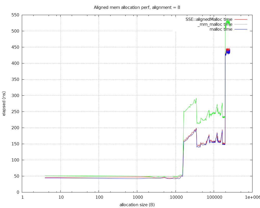
For some reason the aligned memory allocator supplied by VS 2015 is really slow.
See the following results:
SSE::alignedMalloc is our implementation, which works in the standard way - it allocates requested size + alignment, then moves up the returned pointer to so that it is aligned, while storing the original pointer so it can be freed later.
_mm_malloc is the VS function that returns aligned memory. It compiles to a call to the same function as _aligned_malloc.
Finally malloc is of course the standard, boring memory allocation function.
As you can see, for some weird reason, VS's _mm_malloc is much slower than malloc and our aligned alloc implementation (SSE::alignedMalloc).
Actually it's not that common to find a compiler issue that can be replicated with such a small amount of code in my experience, which is kind of satisfying.
Compiling
uint32 bitTest(uint32 y, uint32 N)
{
	int shift = 1;
	for(uint32 i=0; i<N; ++i)
		shift = y >> (shift + 1);
	return shift;
}
In VS2015 update 3, with optimisations enabled, gives
In the Visual Studio 2015 standard library, the implementation of std::map::find is unnecessarily slow.
The underlying reason seems to be similar to that for bug #2 - using operations on a generic tree class that doesn't take advantage of the restrictions places on std::map - that entry keys are unique.
The issue in detail:
std::map::find() calls std::_Tree::lower_bound, which calls _Lbound, which looks like
_Nodeptr _Lbound(const _Other& _Keyval) const
{	// find leftmost node not less than _Keyval
	_Nodeptr _Pnode = _Root();
	_Nodeptr _Wherenode = this->_Myhead();	// end() if search fails

	while (!this->_Isnil(_Pnode))
		if (_Compare(this->_Key(_Pnode), _Keyval))
			_Pnode = this->_Right(_Pnode);	// descend right subtree
		else
		{	// _Pnode not less than _Keyval, remember it
			_Wherenode = _Pnode;
			_Pnode = this->_Left(_Pnode);	// descend left subtree
		}

	return (_Wherenode);	// return best remembered candidate
}
Which is a traversal down a binary tree. The issue is that the traversal doesn't stop when an interior node has a key that is the same as the target key. This is presumably because if you allow multiple entries with the same key, you need to keep traversing to get the leftmost of them. However since we know that entry keys are unique in std::map, the traversal could stop as soon as it traverses to an interior node with matching key.
Proposed fix
The fix is to check the interior nodes keys for equality with the target key, and return from the traversal immediately in that case.
_Nodeptr _Lbound(const _Other& _Keyval) const
{	// find leftmost node not less than _Keyval
	_Nodeptr _Pnode = _Root();
	_Nodeptr _Wherenode = this->_Myhead();	// end() if search fails

	while(!this->_Isnil(_Pnode))
		if(_Compare(this->_Key(_Pnode), _Keyval))
			_Pnode = this->_Right(_Pnode);	// descend right subtree
		else
		{
			// NEW: else node >= keyval
			if(!_Compare(_Keyval, this->_Key(_Pnode))) // NEW: if !(keyval < node):
				return _Pnode; // NEW: then keyval == node, so return it

			// _Pnode not less than _Keyval, remember it
			_Wherenode = _Pnode;
			_Pnode = this->_Left(_Pnode);	// descend left subtree
		}

	return (_Wherenode);	// return best remembered candidate
}
This doesn't change the asymptotic time complexity of the find call, it's still O(log(n)).
But it does somewhat decrease the number of nodes that need to be traversed on average.
It does require additional key comparisons, which could result in a net slowdown in some cases, but the cost of unneeded memory accesses are likely to be higher than the cost of the additional comparisons in most cases, I believe, especially as the number of entries in the map increases and cache misses become more common.
Results with the proposed fix
I implemented the proposed fix above in a class copied from std::map, called modified_std::map.
Doing 1M lookups in a map and modified map with 2^16 unique int keys:
The modified map find method is approximately 15% faster. This isn't a huge amount, but is worth optimising/fixing, for such a commonly-used operation!
How do you tell if an entry with a specific key has been inserted in a std::map and std::unordered_map?
Historically the way was to call find and compare against end, e.g.
if(m.find(x) != m.end()) // If present:
	// do something
With the introduction of C++11, there is another technique - calling count.
if(m.count(x) != 0) // If present:
	// do something
Note also that in std::map and std::unordered_map, count can only return 0 (in the case where the entry is not present) and 1 (when it is). Multiple entries with the same key are not allowed in a map or unordered_map.
You might think that both techniques for testing if an element with a given key is in a map would have similar performance, but this is not the case with some implementations.
What we see is that count takes about twice the time that find does.
Why does count take so long? Stepping through the code in the VS debugger reveals the answer. Count calls equal_range, which computes the range of elements with the same key. equal_range effectively does two tree traversals, one for the start of the range, and one for the end. This is the reason why count takes approximately twice as long (at least for std::map).
I haven't looked into why std::unordered_map::count is slow but I assume it's for a similar reason.
Proposed solution
My proposed solution is to replace the implementation of std::map::count with something like the following:
A few days ago my colleague Yves mentioned a perplexing finding to me - It was significantly faster to call find on a std::unordered_map, and then insert a item into the map only if the find call indicates it is not present, than to just attempt to insert an item directly with an insert call.
This is strange, because the semantics of std::unordered_map::insert are that if an item with a matching key is already in the map, then the item is not updated, and insert returns a value indicating that it failed.
Calling find, then insert, is effectively doing the lookup twice in the case where the item is not in the map already. (and doing the lookup once when it is).
Calling insert directly should only be doing the lookup once, and hence should be of comparable speed or faster.
Here is some code demonstrating the problem:
const int N = 1000000; // Num insertions to attempt
const int num_unique_keys = 65536;

std::unordered_map<int, int> m;
for(int i=0; i<N; ++i)
{
	const int x = i % num_unique_keys;
	if(m.find(x) == m.end()) // If no such entry with given key:
		m.insert(std::make_pair(x, x));
}
Is significantly faster than
std::unordered_map<int, int> m;
for(int i=0; i<N; ++i)
{
	const int x = i % num_unique_keys;
	m.insert(std::make_pair(x, x));
}
Both code snippets result in a map with the same entries.
Perf results:
std::unordered_map find then insert: 0.013670 s, final size: 65536
std::unordered_map just insert:      0.099995 s, final size: 65536
std::map find then insert:           0.061898 s, final size: 65536
std::map just insert:                0.131953 s, final size: 65536
for Visual Studio 2012, Release build.
Note that for std::unordered_map, 'just inserting' is about seven times slower than calling find then insert, when it should be comparable or faster.
std::map also appears to suffer from this problem.
Looking into this, it became apparent quickly that insert is slow, and especially that insert is slow even when it doesn't insert anything due to the key being in the map already.
Stepping through the code in the debugger reveals what seems to be the underlying problem - insert does a memory allocation for a new node (apparently for the bucket linked list) unconditionally, and then deallocates the node if it was not actually inserted! Memory allocations in C++ are slow and should be avoided unless needed.
This seems to be what is responsible for the insert code being roughly seven times slower than it should be.
The obvious solution is to allocate memory for the new node only when it has been determined that it is needed, e.g. only when a matching key is not already inserted in the map.
(There is a related issue as to why chaining is even used in std::unordered_map as opposed to open addressing with linear probing, but I will leave that for another blog post)
Performance of std::map and std::unordered_map can be critical in certain algorithms, so suffering from such massive unneeded slowdowns could be significantly slowing down a lot of code using std::unordered_map.
More results on other platforms
The problem is not fixed in VS2015:
std::unordered_map find then insert: 0.015878 s, final size: 65536
std::unordered_map just insert:      0.096205 s, final size: 65536
std::map find then insert:           0.060897 s, final size: 65536
std::map just insert:                0.128556 s, final size: 65536
Xcode on MacOS Sierra: (Apple LLVM version 7.3.0 (clang-703.0.31)):
std::unordered_map find then insert: 0.020444 s, final size: 65536
std::unordered_map just insert:      0.069502 s, final size: 65536
std::map find then insert:           0.053847 s, final size: 65536
std::map just insert:                0.094894 s, final size: 65536
So the Clang std lib on Sierra seems to suffer from the same problem.
Clang 3.6 I built on Linux: (clang version 3.6.0 (trunk 225608)):
std::unordered_map find then insert: 0.013862 s, final size: 65536
std::unordered_map just insert:      0.015043 s, final size: 65536
std::map find then insert:           0.076331 s, final size: 65536
std::map just insert:                0.092790 s, final size: 65536
The results for this Clang are much more reasonable.
I haven't tried GCC yet.
If you want to try yourself, source code for the tests is available here:
map_insert_test.cpp. You will have to replace some code to get it to compile though.
Summary: Faster-than-light (FTL) communication is traditionally thought to violate causality according to special relativity. However if there is an absolute space and time (absolute reference frame), causality violation is avoided. Instead observers can detect and measure their speed relative to the absolute reference frame.
The standard story
Faster-than-light (FTL) communication is thought by some to allow signalling back in time, thereby violating causality.
(It's worth noting that no FTL communication is actually known to be possible in the real world, however it's interesting from a metaphysical point of view, and also for science-fiction authors!)
It works like this: imagine you have two space stations floating in space, stationary relative to each other (s.s. a and s.s. b on illustration below).
Then imagine you have a rocket that flies past the space stations at some velocity v.
Then imagine that you have some device that can transmit information faster than light; let's suppose that it can transmit with an infinite velocity.
So space station a sends a FTL pulse to space station b. This is the horizontal green line from O to A in the illustration.
As space station b receives the FTL pulse, we've arranged it so that the rocket is at that exact moment flying right past space station b. So space station b communicates with the rocket. (Just with normal light is fine since they are basically at the same position)
Here's the tricky bit: Special relativity says that the rocket has a different coordinate frame than the space stations. In particular the x axis, which corresponds to all the points in space at the same rocket-time, is not the same as the x-axis for the space stations.
So the standard story is that the infinite velocity FTL commuication pulse, sent back from the rocket to the left (lower green arrow from A to B), will travel along the skewed x axis of the rocket-time.
Space station a then receives the pulse at B. Crucially, from the point of view of space station a, it has received the return communication before it sent it!
This is where the paradoxes come in. For example, what if the message said something like 'do not send the message', or 'kill this person, who is the grandfather of the message sender'. Then a contradiction arises.
Much ink has been spilled (or keys mashed) trying to resolve this seeming contradiction.
v:
Interactive illustration - try changing the v value. A depiction of how FTL signalling violates causality in the standard special relativity story. Green lines = FTL communication. Blues lines = trajectory of space stations. Bold red line = trajectory of rocket.
With absolute space and time
With an absolute space and time, sending messages back in time is prohibited. Let us suppose that the space stations are at rest with respect to absolute space. Then the message from the rocket back to space station a does not point down in the space-time plot, but is instead just horizontal. Therefore no contradiction can arise.
v:
Interactive illustration - try changing the v value. A depiction of how causality violation with FTL signalling is avoided with absolute time. Green lines = FTL communication. Blues lines = trajectory of space stations. Bold red line = trajectory of rocket.
What happens instead of a contradiction, is that with FTL communication, you can determine your velocity relative to the absolute reference frame (absolute space).
Imagine a setup where you have two meter rulers, one pointing in the positive x direction, one in the negative x direction. You simultaneously send a FTL pulse to both ends of the rulers. There is a device at each end of the rulers that when it receives the FTL pulse, sends a light pulse back to you.
If you are at rest relative to the absolute reference frame, the light pulses will return to you at exactly the same time. However if you are at motion relative to the absolute reference frame, the light pulses will return at different times. In particular, you will receive the light pulse from a ruler pointing in the direction of travel earlier than the pulse from a ruler pointing away from the direction of travel. See the illustration below.
An observer can calculate their speed relative to the absolute reference frame by measuring the difference in times between the return of the light pulses.
Physicists might refer to this as 'symmetry breaking' - the apparent equality of each reference frame is broken, and you can detect the absolute frame from the comfort of your laboratory.
v:
Interactive illustration - try changing the v value. A depiction of an observer measuring their speed relative to absolute space with FTL signalling. Green lines = FTL communication. Blues lines = light pulses. Red line = world line of observer moving relative to absolute reference frame.
Special relativity and absolute time and space
Special relativity does not eliminate the possibility of an absolute reference frame - rather it is an axiom of special relativity that it is impossible to detect the velocity of the observer relative to any possible absolute reference frame.
It is an additional metaphysical step to discard the undetectable absolute reference frame as non-existing.
To quote Matt Visser:
Warning: the "Einstein relativity principle" does not imply that there's no such thing as "absolute rest"; it does however imply that the hypothetical state of "absolute rest" is not experimentally detectable by any means. In other language, the "Einstein relativity principle" does not imply that the "aether" does not exist, it implies that the "aether" is undetectable. It is then a judgement, based on Occam's razor, to dispense with the aether as being physically irrelevant.
Some further food for thought regarding a potential absolute reference frame that not everyone is aware of - did you know that what is thought to be the afterglow of the Big Bang, called the Cosmic Microwave Background (CMB) is visible in all directions from Earth, and that scientists have measured the speed of the Earth relative to the CMB, which is possible due to the red-shift of the CMB spectrum in the direction of Earth's travel? Earth is travelling at about 0.002c (0.2% the speed of light) through the Universe relative to the CMB. Personally I regard the CMB as some kind of evidence for absolute space and time.
General relativity (the theory of gravity which explains gravity as curvature of space-time) also has profound things to say about space and time, but I have restricted myself to special relativity in this post.
Edit: Added some text in the 'With absolute space and time' section clarifying that the space station is stationary with respect to absolute space.
Added a space-time diagram in the 'With absolute space and time' section to illustrate what I propose would happen with the FTL signals.
This code, which is a gross violation of any reasonable type system, compiles without warning! You can add 10.0f to a boolean value apparently and it's just fine! Of course the reason is that true gets converted to the integer 1, for historical C reasons presumably. And then the resulting value of 11.f effectively gets converted back to a boolean! (to evaluate the condition)
The thing that sucks about C++ in this case is the automatic conversion of true to 1, which allows 10.0f + true to pass the type checker. Automatic conversion/casting of types in a language is very dangerous. Each case should be closely considered by the designer(s). And in this case it's just a bad idea. Fuck you C++.
Edit: This is how our programming language Winter handles it:
AdditionExpression: Binary operator '+' not defined for types 'float' and 'bool'

buffer, line 1:
def main(real x) real : 10.0f + true ? 1.0f : 2.0f
                              ^
If you need to sort some data on the CPU, and you want to do it efficiently, you can do a lot better than std::sort.
For the uninitiated, std::sort is the sort function in the C++ standard library. It's a comparison-based sort, usually implemented as quicksort.
Recently I did some work on a parallel radix sort. A radix sort is not a comparison based sort. Instead it uses the actual values of 'digits' (chunks of bits) of the key to efficiently sort the items. As such radix sorts can run faster than comparison based sorts, both in terms of computational complexity and in practical terms.
Some results
The task is to sort N single-precision float values (32-bit floats). The floats have random values.
For the timings below N = 2^20 = 1048576. Best values from ~10 runs are given. Computer: i7-3770 (4 hardware cores), Platform: Windows 8.1 64-bit, compiler: Visual studio 2012, full optimisations + link time code generation.
std::sort:           0.08427573208609829 s  (12.442205769612862 M keys/s)
tbb::parallel_sort:  0.016449525188363623 s (63.745061817453646 M keys/s)
Radix sort:          0.013582046893134248 s (77.20309083383134  M keys/s)
Parallel radix sort: 0.006327968316327315 s (165.70500160288134 M keys/s)
Note that my parallel radix sort is roughly 13 times faster than std::sort!
Breaking down the speedup over std::sort, it looks something like this:
std::sort -> serial radix sort gives a ~6.2 times speedup.
serial radix sort -> parallel radix sort gives a ~2.1 times speedup.
This is way below a linear speedup over the serial radix sort, considering I am using 8 threads in the parallel sort.
This likely indicates that memory bandwidth is the limiting factor.
Limitations of radix sort
Radix sort is not always the appropriate sorting choice. It has some memory and space overheads that make it a poor choice for small arrays. Once the number of elements gets smaller than 300 or so I have measured std::sort to be faster.
In addition, to be able to radix sort items, you need to be able to convert each key into a fixed length number of bits, where the ordering on the bit-key is the same as the desired ordering.
Therefore you can't sort e.g. arbitrary length strings with radix sort. (Although you could probably use some kind of hybrid sort - radix sort first then finish with a quicksort or something like that)
Conclusion
Parallel radix sort is awesome!
If you are really desperate to sort fast on the CPU and want to use/licence the code, give me an email. Otherwise we'll probably open-source this parallel radix sorting code, once we've got Indigo 4 out the door.
Implementing a parallel radix is also quite fun and educational. I might write an article on how to do it at some point, but writing your own is fun as well!
Take a function \(f\) that maps from some bit string of length \(N\) to another bit string also of length \(N\).
Suppose that this function is a 'hash function' with some properties we want:
1) Given an output value, it takes on average \(2^{N-1}\) evaluations of different inputs passed to \(f\) before we get the given output value. Note that if we try all \(2^N\) different inputs, we will definitely find the input that gives the output we are searching for, if it exists. So we want our hash function to require half than number of evaluations on average before we find it, e.g. \({2^N}/2 = 2^{N-1}\).
2) \(f\) runs in polynomial time on the length of the input \(N\). All practical hash functions have this property.
So let's consider a search problem — call it \(S\). Instances of \(S\) consist of an output string \(y\) (of \(N\) bits length), and the problem is to find the input \(x\) such that \(f(x) = y\).
The first property we are assuming of \(f\) implies that any algorithm that solves this problem runs in time \(2^{N-1}\), which is exponential in \(N\), so not polynomial in \(N\). So \(S\) is not an element of \(P\), the set of problems that are solvable in polynomial time.
Now, let's suppose that we have some proposed input value \(x\). We can verify that \(f(x) = y\) in polynomial time, since we have assumed that \(f\) runs in polynomial time. If \(f(x) \neq y\), the proposed solution will be rejected in polynomial time. This means that we have an algorithm (the verification algorithm) that verifies a proposed solution in polynomial time.
But we know that the complexity class \(NP\) (non-deterministic polynomial) is the class of problems that can be verified in polynomial time. Therefore \(S\) is in \(NP\).
Since we already proved (given our assumptions about \(f\)) that \(S\) is not in \(P\), we therefore have \(P \neq NP\).
So we have the following situation:
The existence of a hash function with the properties we want implies \(P \neq NP\).
Since no-one knows if \(P = NP\), we can deduce that no-one knows if hash functions with the properties we want exist.
Fixed length outputs
Note that this proof only applies for hash functions from strings of N bits to strings of N bits. Some cryptographic hash functions in the real world are defined like this, such as the Skein hash function.
However, most cryptographic functions produce a fixed length output, such as SHA-256 that has a 256 bit output length.
Regardless, I think the same general principle applies. As far as I know, no hash function with a fixed length output has been proved to have the analogous properties as listed above. In other words, no hash function with fixed length output N has been proved to take exponential time on N to find an input that maps to the given output.
One-way functions
This property of hash functions we are thinking about is also called the 'one-way' function property. A hash function with this property is one-way in the following sense: we can compute the output \(f(x)\), from the input \(x\), easily and efficiently. However going in the 'other direction', e.g. computing the inverse, \(f^{-1}(y)\), is not computable efficiently.
Remarkably we don't know if such one-way functions exist.
Implications
The implication of the above proof and comments is that no-one knows if cryptographic hash functions like the SHA hash functions really have the secure properties that people hope they do.
Many aspects of modern software depend on such hash functions, such as message authentication codes, code signing of executables, and even systems such as bitcoin, which uses the SHA-256 hash function in its proof-of-work scheme.
That these hash functions are not proved to be cryptographically secure is somewhat well known, but it's not that uncommon to hear people assuming that the security or properties of such systems have actually been proved.
This is quite similar to the situation with factoring of large numbers which is used in public key cryptography, which is suspected, or commonly treated as if it is not solvable in polynomial time, even though it has not been proved.
In this blog post I'm going to write a little bit about permutations, and some connections with information theory and sorting algorithms, including giving a sketch-proof of the \(n \log n\) lower bound on comparison-based sorting.
A permutation is a re-ordering of a list.
For example, (1, 3, 2), (3, 2, 1) and (2, 1, 3) are all permutations of the list (1, 2, 3).
Let's say you have a list with \(n\) elements in it (e.g. the length of the list is \(n\)). How many different ways of ordering the list (e.g. how many permutations) are there of the list?
When picking the first element of your permutation, you have n elements to choose from. Pick one. Then when picking the 2nd element of your permutation, you have one less to choose from, e.g. \(n-1\) elements. By the time you come to choose the last element of your permutation, you only have one element left. So the total number of different permutations is
$$n \times (n - 1) \times (n - 2) \times ... \times 3 \times 2 \times 1 $$
This is the definition of n factorial:
$$n! = n \times (n - 1) \times (n - 2) \times ... \times 3 \times 2 \times 1$$
So there are \(n!\) permutations of a list of n elements.
Let's say we want to store which permutation we have chosen in computer memory. Since there are \(n!\) possibilities, we need to use \(\log_2(n!)\) bits to store this information.
(In general, to store a choice that has x possibilities, you need to use \(\log_2(x)\) bits. For example, with 256 possibilities, you need to use \(\log_2(256) = 8\) bits.)
Once of the most important features of the log function, is the following rule - the 'log of products' is the 'sum of the logs'. In other words,
$$\log(a \times b) = \log(a) + \log(b)$$
Let's have a look at the expression \(\log_2(n!)\), and substitute in the definition of \(n!\):
$$\log_2(n!) = \log_2(n \times (n-1) \times (n-2) \times ... \times 2 \times 1)$$
Using the rule above to break up the log:
$$\log_2(n!) = \\
\log_2(n \times (n-1) \times (n-2) \times ... \times 2 \times 1) = \\
\log_2(n) + \log_2(n-1) + \log_2(n-2) + ... + \log_2(2) + \log_2(1)
$$
The last line can be interpreted in an interesting way - it gives the number of bits required when storing each element choice for the permutation separately.
For example, \(\log_2(n)\) is the information needed to store the first choice, which was from \(n\) options.
\(\log_2(n-1)\) is the information needed to store the second choice, which was from \(n-1\) options.
\( \log_2(1) \) is the information needed to store the last choice, which only has 1 option, e.g. there was no choice for it. Happily, \(\log_2(1) = 0\). No information is needed for this null choice!
This is one of the main reasons (perhaps the only reason?) why the log function pops up in information theory. When you have two independent choices to make, the number of possibilities is the product of the two numbers of possibilities for each choice. But the information required for both is the sum of the two individual pieces of information. The log function is the only function with this property.
Sorting algorithms
The task of a sorting algorithm is to take a permutation of some original sorted list, and return the original sorted list.
Consider a comparison based sorting algorithm, that at each step can compare two elements together with the less than (<) operator. At each step it can eliminate up to half of the possible permutations. In other words, it can gather one bit of information with each comparison.
So to gather all the bits of information needed to determine which permutation it is looking at, it needs to make \(\log_2(n!)\) comparisons.
It could do it less efficiently, but this is the lower bound on the number of comparisons which can handle the worst case.
(This is a very hand-wavy 'proof', but I hope you get the general idea)
Stirling's approximation
Stirling's approximation tells us that
$$\ln(n!) \approx n \ln(n) - n$$
Here \(\ln(x)\) is the natural logarithm function, e.g. \(\log\) with base \(e\).
We can convert natural logarithms to log base 2 by dividing the log function by \(\ln(2)\), which is about 0.6931, e.g.
$$\log_2(x) = \ln(x) / \ln(2)$$
or
$$\log_2(x) \times \ln(2) = \ln(x)$$
Using this rule in previous equation gives:
$$\ln(n!) \approx n \ln(n) - n \\
\log_2(n!) \times 0.6931 \approx n \log_2(n) \times 0.6931 - n \\
\log_2(n!) \approx n \log_2(n) - n / 0.6931
$$
When you are doing asymptotic complexity analysis, constants don't matter.
So the optimal asymptotic complexity of the comparison based sort algorithm
is \(n \log_2(n)\), which is the same asymptotic complexity as \(n \ln(n)\).
Let's look at some actual data points. For \(n = 10\):
One interesting thing to note is that n*log_2(n) is quite a poor estimate of the number of comparisons needed (it is quite a lot too large), at least for these relatively small n values. the (ceiling'd) log_2(n!) values give the actual number of comparisons needed.
So there you go, some curious things about permutations and sorting. I hope some people found this interesting. If there are any bits of maths that you don't understand, let me know and I will go into more depth. Corrections welcome of course.
I sent this email to the Putty guys, but I haven't heard back from them. So I'll post it here.
---------------------------
First of all, thanks for your work on Putty. It's a very useful tool for us.
However pscp uploads much more slowly than it should for us.
We are uploading from our office network (UK) to a server in a German data centre.
Ping latency to the server is ~31ms.
Uploading a ~100MB file, putty stabilises at around 220kB/s:
IndigoRenderer_x64_4.0.14 | 100580 kB | 218.2 kB/s | ETA: 00:00:43 | 91%
The computer it is running on is running Windows server 2008, on an i7-2600, with 16GB RAM.
In comparison, scp running on a Linux machine on the same LAN, uploading to the same server, gets around 8MB/s upload speed.
speedtest.net shows a ~60Mb/s upload speed from our office.
This indicates to me that the pscp upload speeds are a lot slower than they could be.
Is this a problem you are aware of? Are there any plans to improve the upload speed?
Such programs are super annoying. I had this problem on my computer - some program is occasionally stealing window focus, resulting in being switched out of full-screen games at inopportune times etc..
I figured out the offending program is C:\Users\nick\AppData\Local\Akamai\installer_no_upload_silent.exe.
Dear Akamai: please fix your annoying program to not steal window focus. Thank you.
I have looked at this program that presumably does the same thing: http://www.happydroid.com/focus, but Windows Defender said it had a virus in it. Not sure if that is true, but I'm hesitant to run unsigned executables from random sources anyway. So I made my own.
The counts buffer for each thread has 8 x 8 byte elements.
Each thread sees a range of the overall count buffer.
The odd thing is, is that the per-thread count table is 64 bytes already, which is the cache-line size (unit of cachable memory) of modern CPUs.
This means that the count tables for each thread are on different cache lines.
Edit: I was careful to align the per-thread count table to 64 bytes as well.
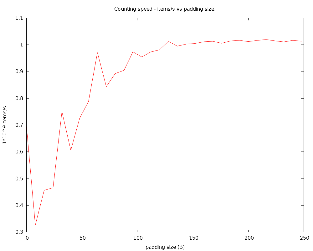
However when I added a large amount of padding between the count tables, the performance shot up.
I made a graph of padding between each 64-byte table:
The peaks are at 0 B, 32 B, 64 B, 96 B, 128 B etc..
So it seems that to avoid false sharing effects, you need quite a lot of padding between data - something like 128 bytes, much more than the zero bytes indicated in almost all online sources.
In other words, it's not enough to just separate the cache lines that each thread works on, they must be separated by several cache-line widths.
Has anyone else seen or know about similar behaviour?
CPUs are very complicated so it's possible I may be seeing some other effect, or there may be a bug in my code.
I saw a comment somewhere that the effect may be due to prefetching of adjacent cache-lines by the CPU, this may be an explanation.
Edit: Here's some C++ source code to demonstrate this effect. This is not the source used to generate the above graph, but is similar to it, and uses C++11 threading, timing etc..
padding: 0 B, elapsed: 0.0312501 s
padding: 8 B, elapsed: 0.0781306 s
padding: 16 B, elapsed: 0.0625087 s
padding: 24 B, elapsed: 0.062502 s
padding: 32 B, elapsed: 0.0312535 s
padding: 40 B, elapsed: 0.0625048 s
padding: 48 B, elapsed: 0.0312495 s
padding: 56 B, elapsed: 0.0312519 s
padding: 64 B, elapsed: 0.015628 s
padding: 72 B, elapsed: 0.0312498 s
padding: 80 B, elapsed: 0.0156279 s
padding: 88 B, elapsed: 0.0312538 s
padding: 96 B, elapsed: 0.0156246 s
padding: 104 B, elapsed: 0.0156267 s
padding: 112 B, elapsed: 0.0156267 s
padding: 120 B, elapsed: 0.0156265 s
padding: 128 B, elapsed: 0.0156309 s
padding: 136 B, elapsed: 0.0156219 s
padding: 144 B, elapsed: 0.0156246 s
padding: 152 B, elapsed: 0.0312559 s
padding: 160 B, elapsed: 0.0156231 s
padding: 168 B, elapsed: 0.015627 s
padding: 176 B, elapsed: 0.0156279 s
padding: 184 B, elapsed: 0.0156244 s
padding: 192 B, elapsed: 0.0156258 s
padding: 200 B, elapsed: 0.0156261 s
padding: 208 B, elapsed: 0.0312522 s
padding: 216 B, elapsed: 0.0156265 s
padding: 224 B, elapsed: 0.0156264 s
padding: 232 B, elapsed: 0.0156267 s
padding: 240 B, elapsed: 0.0156249 s
padding: 248 B, elapsed: 0.0156276 s
It looks like VS2012's 'high resolution' (std::chrono::high_resolution_clock) clock is not actually high resolution, so feel free to replace the timing code with a proper high-resolution clock.
I used our QueryPerformanceCounter-based timer in the original code.
"Streamer - Loads data or instructions from memory to the second-level cache. To use the streamer, organize the data or instructions in 128 bytes, aligned on 128 bytes. The first access to one of the two cache lines in this block while it is in memory triggers the streamer to prefetch the pair line."
Maybe my CPU (i7 Ivy Bridge) is fetching both the cache lines to the left and to the right of the actually used cache line. This would explain the 128-byte padding seemingly needed for optimum performance.
Accessing data through a layer of indirection has some performance impact. The most important aspect of the performance impact however, is if the indirection is predictable.
If the ultimately accessed data is accessed in a coherent order, even through a layer of indirection, performance is still pretty good.
Some results of the code below, which tests 2^26 memory reads done in various ways:
Data size: 256.000 MB
no indirection elapsed:        0.02169 s (12.38 GiB/s, 1.196 cycles/read)
sum: 4261412864
predictable indices elapsed:   0.03996 s (6.718 GiB/s, 2.203 cycles/read)
sum: 4261412864
unpredictable indices elapsed: 0.9277 s (0.2894 GiB/s, 51.15 cycles/read)
sum: 4261412864
As you can see, adding a layer of indirection has some performance impact (~2.2 cycles per read instead of ~1.2 cycles.).
However, as long as the accessed data is accessed in a predictable, coherent fashion, then the cache and prefetcher on the CPU means the slowdown is not too bad.
If, however, the order of access is not coherent and predictable, performance takes a nose-dive, as the CPU cache and prefetcher cannot effectively fetch memory before it is needed or efficiently when it is need, and massive latency is incurred.
This kind of performance degradation is what I expect from unpredictable and incoherent memory access, with or without a layer of indirection.
The key point is that it's not indirection per se that is slow, but unpredictable and incoherent memory access patterns that are commonly seen with indirection.
const int N = 1 << 26; // num reads
const double cycles_per_sec = 3.7e9; // For my i7 Ivy bridge, running in 'turbo-boost' mode.

// Allocate some data, fill with semi-random values.
std::vector<uint32> data(N);
for(int i=0; i<N; ++i)
	data[i] = i % 128;

conPrint("Data size: " + getNiceByteSize(N * sizeof(uint32)));

// Test data access without indirection
{
	Timer timer;
	uint64 sum = 0;
	for(int i=0; i<N; ++i)
	{
		sum += data[i];
	}

	double elapsed = timer.elapsed();
	const double bytes_per_sec = 4 * N / elapsed;
	const double cycles_per_read = (elapsed * cycles_per_sec) / N; // num cycles = elapsed * cycles-per-sec
	conPrint("no indirection elapsed:        " + doubleToStringNSigFigs(elapsed, 4) + " s (" + doubleToStringNSigFigs(bytes_per_sec * 1.0e-9, 4) + " GiB/s, " + doubleToStringNSigFigs(cycles_per_read, 4) + " cycles/read)");
	printVar(sum);
}

// Test indirection with predictable indices
{
	std::vector<uint32> indices(N);
	for(int i=0; i<N; ++i)
		indices[i] = i;

	Timer timer;
	uint64 sum = 0;
	for(int i=0; i<N; ++i)
	{
		sum += data[indices[i]];
	}

	double elapsed = timer.elapsed();
	const double bytes_per_sec = 4 * N / elapsed;
	const double cycles_per_read = (elapsed * cycles_per_sec) / N;
	conPrint("predictable indices elapsed:   " + doubleToStringNSigFigs(elapsed, 4) + " s (" + doubleToStringNSigFigs(bytes_per_sec * 1.0e-9, 4) + " GiB/s, " + doubleToStringNSigFigs(cycles_per_read, 4) + " cycles/read)");
	printVar(sum);
}

// Test indirection with unpredictable indices
{
	std::vector<uint32> indices(N);
	for(int i=0; i<N; ++i)
		indices[i] = i;

	// Permute indices
	for(int t=N-1; t>=0; --t)
	{
		int k = (int)(rng.unitRandom() * t);
		mySwap(indices[t], indices[k]);
	}

	Timer timer;
	uint64 sum = 0;
	for(int i=0; i<N; ++i)
	{
		sum += data[indices[i]];
	}

	double elapsed = timer.elapsed();
	const double bytes_per_sec = 4 * N / elapsed;
	const double cycles_per_read = (elapsed * cycles_per_sec) / N;
	conPrint("unpredictable indices elapsed: " + doubleToStringNSigFigs(elapsed, 4) + " s (" + doubleToStringNSigFigs(bytes_per_sec * 1.0e-9, 4) + " GiB/s, " + doubleToStringNSigFigs(cycles_per_read, 4) + " cycles/read)");
	printVar(sum);
}
bit_cast<T>(x) would get the bits of x, and reinterpret them as the bits of a value of type T.
For example, you would be able to write
float x = 1.0f;
const uint32_t y = bit_cast<uint32_t>(x);
And then y would have the value 0x3f800000.
From a generated-code point of view this would be a no-op. (Or maybe some instructions would have to be emitted for moving to/from floating point registers in this case?)
Edit: A bit_cast is only valid if the source and destination types are the same size. Using bit_cast on types differing in size would give a compile-time error.
This kind of bit conversion needs to be done pretty often if you are writing low-level, high peformance code, or networking code.
There are a number of ways to do something similar with C++ today, but they all have problems, either with correctness or elegance.
Current option 1: pointer casting
Possibly the most old-school way is to pointer cast, like this:
float x = 1.0f;
const uint32_t y = *(uint32_t*)&x;
The problem here is that it is undefined behaviour to write through one pointer type (float*) and read through another (uint32_t*). (due to aliasing rules). Compilers may whinge about it and/or generate code that does not do what you want.
For example, GCC says
"warning: dereferencing type-punned pointer will break strict-aliasing rules [-Wstrict-aliasing]"
(see code example here: https://goo.gl/wZcV2D).
Current option 2: union abusing
The trick here is to write into one of the union fields, then read from the other one.
float x = 1.0f;

union fi_union
{
	float f;
	uint32_t i;
};

fi_union u;
u.f = x;
const uint32_t y = u.i;
This *may* work in practice, but is syntactically ugly, is an abuse of the idea of unions, and may be undefined behaviour.
Current option 3: memcpy
The idea here is to just memcpy() from the src to the dest, and rely on the compiler to recognise what you are doing, and to not actually emit the memcpy function call.
Example:
template <class Src, class Dest>
inline Dest bit_cast(const Src& x)
{
	static_assert(sizeof(Src) == sizeof(Dest), "sizeof(Src) == sizeof(Dest)");
	Dest d;
	std::memcpy(&d, &x, sizeof(Dest));
	return d;
}
This works well in practice, but is a little dangerous in the sense that you are relying on a compiler optimisation to avoid very slow code (e.g. it would be very slow if a function call was actually emitted).
Current (non-)option 4: static_cast
static_cast does not do what we want.
float x = 1.0f;
const uint32_t y = static_cast<uint32_t>(x);
puts the value '1' in y, not 0x3f800000 as we want.
Current (non-)option 5: reinterpret_cast
To be honest I'm not sure what reinterpret_cast is for. I never use it. It also doesn't do what we want:
float x = 1.0f;
const uint32_t y = reinterpret_cast<uint32_t>(x);
gives, in Visual Studio 2012:
"error C2440: 'reinterpret_cast' : cannot convert from 'float' to 'uint32_t'
Conversion is a valid standard conversion, which can be performed implicitly or by use of static_cast, C-style cast or function-style cast"
Semantics
(Added in an edit)
The bit_cast would give the same result as the bit_cast function above:
template <class Src, class Dest>
inline Dest bit_cast(const Src& x)
{
	static_assert(sizeof(Src) == sizeof(Dest), "sizeof(Src) == sizeof(Dest)");
	Dest d;
	std::memcpy(&d, &x, sizeof(Dest));
	return d;
}
Because we know 'd' (the destination) is in a different memory location from 'x' (the source), there shouldn't be any aliasing problems.
Conclusion
So in conclusion, the alternatives are basically hacky workarounds to something missing in the original language. Older alternatives are increasingly rendered invalid due to fussier optimising compilers. I think the problem should be solved once and for all with a built-in language feature - bit_cast.
Winter now has proper runtime support for first class functions, and anonymous functions (lambda expressions) with lexical closures.
A simple example:
def main() float :
	let
		f = \(float x) : x*x
	in
		f(2.0)
returns 4.0.
In this example an anonymous function (that computes the square of its argument) is created and assigned to f. It is then called with the argument 2.0.
Since functions are 'first class', they can be returned from functions:
def makeFunc(float x) function<float> : \() : x
def main() float :
	let
		f = makeFunc(2.0)
	in
		f()
In this example makeFunc returned a function.
To support lexical scoping, variables are captured:
def makeFunc() function<int, int> :
	let
		a = [10, 11, 12, 13]va
	in
		\(int x) int : a[x]

def main(int x) int :
	let
		f = makeFunc()
	in
		f(x)
In the example above the anonymous function returned from makeFunc() captures the variable-length array a, which is indexed into when the function is actually called with f(x).
Closures are allocated on the heap by default. If they can be proven not to escape the current function (which is currently computed with a simple type-based escape analysis), they are allocated on the stack.
The runtime layout for a closure looks like this currently (in LLVM IR):
It has 5 fields: a refcount, some flags (stack or heap allocated), the function pointer, a destructor pointer for cleaning up the captured vars, and a structure containing the captured vars.
All this abstraction doesn't have to come at the cost of runtime inefficiency. Take this program:
def main(array<float, 4> a, array<float, 4> b) array<float, 4> : map(\(float x) : x*x, a)
He notes that only Haskell gets it right. (Maybe Rust got it right since then?)
Winter gets it right as well - strings are treated as sequences of Unicode chars, not sequences of bytes. The encoding (UTF-8) is a hidden implementation detail.
I have reached an interesting milestone in our functional programming language Winter - Winter now can do auto-parallelisation, auto-vectorisation, and even both at the same time :)
Auto-parallelisation means that code is automatically executed in parallel in multiple threads. Auto-vectorisation means that vector (SIMD) instructions are automatically used instead of scalar instructions. This means that e.g. 4 or 8 multiplications can be done with one instruction.
Taking some Winter code, which applies a function to an input array, generating a result array:
def square(float x) float : x*x
def main(array<float, 268435456> a, array<float, 268435456> b) array<float, 268435456> :
    map(square, a)
We're using a large array size here so we get a decent, measurable amount of work to do.
Very nice code here, LLVM is doing a good job. You can see there are 4 256-bit memory loads being done in parallel, then 4 256-bit 8-element multiplications being done in parallel, then 4 stores being done.
This code runs at memory speed, which is about 5.7 GB/s in this case on my machine. Even a much sloppier inner loop will still run at memory speed when there is this little work to do per element.
Resulting perf measurements are:
JITed code elapsed: 0.187149 s
JITed bandwidth: 5.73737 GiB/s
C++ ref elapsed: 0.196158 s
C++ ref bandwidth: 5.47385 GiB/s
Both the JITed Winter code and the C++ code are memory limited so run at similar speeds.
Taking another example, where more work is done per array element:
def f(float x) float : pow(x, 2.2)
def main(array<float, 268435456> a, array<float, 268435456> b) array<float, 268435456> :
    map(f, a)
pow() is a pretty slow function (100 cycles or more). This allows us to see the influence of auto-parallelisation.
Winter auto-parallelises this map function, dividing the array into slices, and passing each slice to a worker thread, on which the actual work is done.
With auto-parallelisation disabled, results are as follows:
pow(x, 2.2), single threaded map():
JITed code elapsed: 6.32286 s
JITed bandwidth: 0.169819 GiB/s
C++ ref elapsed: 1.90434 s
C++ ref bandwidth: 0.563838 GiB/s
The reason the C++ version is faster, is because Visual C++ vectorises the pow() function, whereas LLVM doesn't (I just filed a bug report on this here.)
With auto-parallelisation enabled:
pow(x, 2.2), multi threaded map()
JITed code elapsed: 1.35347 s
JITed bandwidth: 0.793327 GiB/s
C++ ref elapsed: 1.94178 s
C++ ref bandwidth: 0.552969 GiB/s
You can see from the highlighted result that the program runs about 4.67x faster, which is roughly what you would expect using 8 threads on 8 logical cores, considering that 4 of them are hyperthreading cores.
No changes in the winter code were required to use this parallelisation, it's completely automatic.
So there you have it - a proof-of-concept of auto-vectorisation and auto-parallelisation in Winter. The code is not robust yet - I just got it working this weekend. But I think it's quite a promising result. It also shows, I think, that functional programming languages can be just as fast (or faster) than optimised, multithreaded C++ code.
I have spent the last week or so fixing bugs in Winter (our programming language) found by our new fuzz testing code.
Fuzz testing is the process of sending lots of random input to a program, to try and uncover crashes or other undesirable behaviour from the program.
If you are writing a compiler, I highly recommend fuzz testing it, it seems like a very effective way of finding bugs.
Some more details about our fuzzing code:
It's an in-process fuzzer - random programs are generated, compiled, and run if compilation succeeded (e.g. if the program is valid), all in the same process.
Because it's in-process, as soon as a crash occurs, the fuzzing run is over. Each random program string is saved to disk before it is run, so to find the program that crashed the process, you just have to get the last line from the file on disk.
It's multithreaded, because you need all the power you can get to find any bugs as fast as possible.
The fuzzer runs through about 20,000 random programs per second per core, so running on 4 cores gives around 80,000 random programs per second.
This relatively fast speed is possible because invalid programs are rejected early before computationally intensive stuff like LLVM optimisation and codegen starts.
Valid programs only run at about 300 programs per second per core, but most random programs are invalid, so the average speed comes out to 20K/core/s
The random program generation strategy is something like:
Randomly pick a program from the unit test suite programs (several hundred covering all language features)
Then repeatedly mutate program randomly a few times by picking from among a few options:
1) Insert a random character at a random position in the program.
2) Delete a random chunk of characters from the program
3) Copy a chunk of the program to another random position in the program.
4) Read a section of a random other program from the test suite and insert into the program.
5) Insert a random language keyword or syntactical elements (square bracket pair etc..)
As mentioned I found this fuzzing code to be extremely effective in finding bugs. I found 40-50 crash bugs that took something like a week to fix, and triggered improvements and refactorings to avoid crashes. Our programming language Winter is a lot more robust now.
if you are wondering how there can be so many bugs in a language compiler/runtime, bear in mind that Winter is quite complex, with generic functions, operator overloading, function overloading, type coercion, JITing, higher order functions etc..
I also tried out American Fuzzy Lop (AFL). I ran it for 24 hours or so, in which time it got through 20% or so of the first pass. It didn't find any crashes.
I'm not sure if this is because it's not very good at finding crashes, or if I removed all the crash bugs :)
It's definitely a lot slower than our in-process multithreaded fuzzing though.
Note that in theory AFL uses a more powerful kind of fuzzing - coverage-guided fuzzing, which can be considered a white-box approach, since it uses knowledge of what code paths are taken for each input program.
Therefore I would highly recommend integrating an in-process fuzzer into your test suite, and after that maybe check out AFL or similar.
(If you want to know more about Winter there are some presentation slides in PDF format from a talk I gave a while ago here: Indigo Shader Language and Winter)
Assume, for a contradiction, that we have some function optimise(f), that returns the fastest Turing Machine that computes the (partial) function f.
The exact definition of 'fastest' doesn't matter.
Now consider the function \( \operatorname{returnOneOnHalt_f}(x) \), that simulates the execution of function f on input x. If f halts, then \( \operatorname{returnOneOnHalt_f} \) returns 1 and halts. If the function f doesn't halt then \( \operatorname{returnOneOnHalt_f} \) doesn't halt.
Now consider what happens when we run optimise() with \( \operatorname{returnOneOnHalt_f} \) as input, e.g. \( \operatorname{optimise}( \operatorname{returnOneOnHalt_f} \)).
For a given function f, if f halts on all inputs, then \( \operatorname{returnOneOnHalt_f}(x) = 1 \).
Therefore the fastest Turing machine that computes this function is the one that just writes 1 to the tape and then halts.
On the other hand, if f does not halt on all inputs, then there is at least one input value for which the optimsed \( \operatorname{returnOneOnHalt_f}\) does not halt. This Turing machine is more complex than the machine that just writes one and halts. For example it will execute more than one step as it does not halt.
Therefore we have created an effective procedure for determining if f halts on all inputs - just look at the optimised \( \operatorname{returnOneOnHalt_f} \) and see if it is the 'write one to tape and halt' machine.
However we know that such an effective procedure is impossible due to the Halting Theorem. Therefore we have a contradiction, and we cannot have such a function optimise().
Pseudocode for such a procedure looks like this:
function makeReturnsOneOnHalt(f)
	return function that simulates f, and when f halts, returns 1.
end

function doesHaltOnAllInputs(f)
	returnsOneOnHalt_f = makeReturnsOneOnHalt(f)

	optimised_returnsOneOnHalt_f = optimise(returnsOneOnHalt_f)

	return optimised_returnsOneOnHalt_f == returnsOne
end
Consequences for superoptimisation
Superoptimisation is a compiler optimisation technique that is supposed to find the shortest, or fastest program to compute a function. In other words, it doesn't just make a program somewhat faster, but actually finds the optimal program.
If the programs being considered are 'Turing-complete' (or 'Turing-machine equivalent'), then either kind of superoptimisation (optimising for program length of for program speed) become impossible (uncomputable).
Finding the shortest program is uncomputable as a consequence of Kolmogorov Complexity theory.
As the proof above demonstrates, finding the fastest program that computes a given function is also uncomputable.
This means that superoptimisation must necessarily be restricted to subsets of all possible functions, such as the total functions.
Multiplication in C++ is left to right associative - e.g.
y = a * b * c
means
y = (a * b) * c
Note that although the mathematical operation of multiplication is associative, e.g. (a * b) * c = a * (b * c), the same is not true for floating point multiplication, due to intermediate rounding error.
Therefore in default circumstances, the compiler may not optimise
y = a * b * c
to
y = a * (b * c)
as it may give different results.
However, if 'fast math' mode is enabled, compilers may in theory perform this 'reassociation'.
This can be important for a number of reasons - one is that b and c may be constants, and the y = a * (b * c) may be inside a loop. Performing reassociation means that the b*c multiplication may be 'hoisted' outside the loop, so only one multiplication is done instead of two.
Clang performs this reassociation optimisation:
float f()
{
  	const float b = 2.f;
	const float c = 3.f;
	float sum = 1.f;
	for(int i=0; i<1024; ++i)
	{
		const float a = (float)(sum + 1.f);

		const float y = a * b * c;
		sum += y;
	}

  return sum;
}
Although VS has unrolled the loop a bit, you can see that there are two multiplications done, with a dependency between them, e.g. the first has to finish before the second is done.
So VS doesn't seem to do the reassociation optimisation, even with fast maths enabled (/fp:fast), which is unfortunate.
The RDTSC instruction on x86 CPUs is supposed to read a counter that is incremented (by one) every clock cycle.
However, it doesn't actually do this. Instead, the counter increases at a fixed frequency, independent of the actual clock speed of your CPU,
which varies based on load, temperature etc..
This does not seem to be documented anywhere. I found this out the hard way, after measuring the frequency of rdtsc myself, and noticing it differs from that given by CPU-z.
The CPU-z value seems greatly more likely to be the correct value, since it correlates with temperature values of the CPU (reported with speedfan) and actual amount of work done by the CPU (speed of execution of a program).
On my i7 920, which has a 'on the box' clock speed of 2.67 GHz, RDTSC increments at ~2.664 GHZ.
The actualclock speed varies from 1.5 GHz at idle, to ~2.8GHz under load (measured with CPU-z).
In summary: some idiot at some point got confused by changing clock speeds, and complained as it broke their dodgy program, so AMD and Intel changed the semantics of RDTSC to run at a fixed freq.
Meanwhile I found out completely by accident after several years of using RDTSC.
To me this is good example of the terrible situation modern computer and software 'engineering' is in. Changes of semantics like this are not documented properly, or even at all, and you only find out years
later by accident, and can only confirm it and find an explanation in some random stack overflow post.
Pretty much everyone disagreed with me. Oh well, such is life.
My central point in that article was that it matters which language we use. For any given string, there is a language such that the Kolomogorov complexity of the string with respect to the language is zero. This means that Kolomogorov complexity tells us nothing useful about if some given string is 'random' or not.
The invariance theorem
Some people brought up the invariance theorem in defense of some global notion of Kolmogorov complexity. While the theorem may be true, what it says is basically useless in trying to define a global Kolmogorov complexity - i.e. a complexity that is independent of the language chosen.
Let's walk through an example of how the invariance theorem fails to do anything helpful. I'll use the notation from my previous post.
First a definition of the invariance theorem (from Wikipedia):
If \( K_1 \) and \( K_2 \) are the complexity functions relative to Turing complete description languages \(L_1\) and \(L_2\), then there is a constant \(c\) – which depends only on the languages \(L_1\) and \(L_2\) chosen – such that
$$ \forall s. -c \le K_1(s) - K_2(s) \le c $$
The proof follows from considering an interpreter for \(L_1\) written in \(L_2\) and vice-versa.
Ok, so that's the invariance theorem. Now lets work through an example of why it is useless. Consider some arbitrary string \(x\), for example:
$$ x=ababaaabbabaabaababbbabaababbbaaababbbba $$
Let us suppose the complexity wrt. language \(L_1\) is 20, e.g.
$$ K_1(x) = 20 $$
Now consider the language \(L_{silly, x}\), defined as in the previous post. This is the language specifically chosen to make the complexity of x zero in the language. From the definition of \(L_{silly, x}\), we have
$$ K_{silly, x}(x) = 0 $$
So, what does the invariance theorem say about the two languages we have chosen? (\(L_1\) and \(L_{silly, x}\))
The invariance theorem says that there is some constant \(c\) such that
$$ \forall s. -c \le K_1(s) - K_{silly, x}(s) \le c $$
or using our values \(K_1(x) = 20\) and \(K_{silly, x}(x) = 0\): (since the statement holds for all strings)
$$ -c \le 20 - 0 \le c $$
so
$$ -c \le 20 \le c $$
so
$$ c \ge 20 $$
In other words, for this particular string \(x\), there is some language \(L_{silly, x}\) such that the complexity of x wrt. the language is zero, and the bound (\(c\)) for this pair of languages is large enough to cover the gap in complexities between the two languages. So the invariance theorem has not stopped the complexity of \(x\) going to zero in some other language, even though it is non-zero in \(L_1\).
An alternative definition of Kolmogorov complexity
There are alternative definitions of Kolmogorov complexity, for example the one
by given by Peter Bro Miltersen in his course notes.
These alternative definitions also suffer from the same problem - the complexity depends on the language chosen, and there is no reasonable 'invariant' complexity.
Recapping his definitions, we have programming systems (languages) \(L\), and programs in these languages: \(p \in L\). These are given semantics in the following way:
Each language \(L\) has two associated algorithms \(\phi\), \(\tau\) so that \(\phi(p)\) for \(p \in L \) outputs the index of a Turing machine \(M_{\phi(p)}\). So \(p\) is given the behavior of the associated Turing machine:
$$ p(x) := M_{\phi(p)}(x) $$
A Kolmogorov decoder relative to L is then defined:
$$ d_K(pz) := p(z) $$
This function works by splitting the string \(pz\) into two components - the description of the program \(p\), and the input to the program, \(z\). For this to work, no program string \(p\) can be the prefix of another one.
The Kolmogorov code is then defined:
$$ c_K(x) := \text{the shortest y so that } d_K(y) = x $$
Note that in in this definition \(y\) is not a program, but the definition of a program along with input to the program, concatenated together.
Finally the Kolmogorov complexity is given as
$$ K(x) := |c_K(x)| $$
e.g. the length of the Kolmogorov code.
Using these definitions, we can make the following theorem:
Theorem: For any finite string \(x\), there is some language \(L_{silly, x}\) such that the Kolmogorov complexity of \(x\) in \(L_{silly, x}\) is 1.
Proof:
For the given string \(x\), there is some Turing machine that outputs \(x\) then halts, when given the empty string input \(\varepsilon\). Suppose this Turing machine has index i.
Define the associated semantics algorithm \(\phi\) for the language such that
$$ \phi(p_1) := i $$
Where
$$ p_1 = ``1" $$
E.g. \(p_1\) is the string \(``1"\).
Which means that
$$ p_1(\varepsilon) = M_{\phi(p_1)}(\varepsilon) = M_i(\varepsilon) = x $$
So
$$ d_K(p_1\varepsilon) = p_1(\varepsilon) = x $$
Given that
$$ c_K(x) = \text{the shortest y so that} d_K(y) = x $$
we have
$$ c_K(x) = p_1\varepsilon$$
$$ c_K(x) = ``1" $$
so
$$ K(x) := |c_K(x)| = 1 $$
The reason we have a complexity of one instead of zero is due to the prefix-free property required when combining the two strings for \(d_K\).
Let's say we have some (total) function \(f\), defined on some finite domain \(A\):
$$ f : A \mapsto B $$
For example, f might be a square function defined on \( \{1, 2, 3, 4\} \):
Input    Output
1        1
2        4
3        9
4        16
The question now arises, is it possible to define an effective procedure that will determine the fastest Turing machine that computes the function \(f\).
Without any limitations on the Turing machine, we can simply construct a Turing machine that computes f in one step - you basically encode f into the transition function of the Turing machine.
Theorem: There is an effective procedure for finding the fastest Turing machine that computes a function f with finite domain. The fastest Turing machine takes just 1 step.
Proof: To do this we construct a machine \(T_1\) that has a different tape symbol for each input value to the function - e.g. element in the domain \( A \). The transition function of \(T_1\) then simply maps from the read element \(a\) to the output element \( f(a) \). The machine \(T_1\) writes \( f(a) \) to the tape, overwriting \( a \), then halts.
Q.E.D.
I don't find this a very interesting proof, since it doesn't really follow the ethos of Turing machines - which it violates by throwing more table symbols at the problem until it can do it in one step. A more interesting problem is the case where the tape alphabet \( \Gamma \) is fixed - e.g. to the binary case, where it consists of just the set \( \{0, 1, b\} \) - zero, one, and blank. This corresponds a lot better to 'real' computers.
So let's fix the tape alphabet and ask the question again:
Given a fixed tape alphabet \( \Gamma \), is there an effective procedure for finding the fastest Turing machine that computes the given function \(f\), where \(f\) has a finite domain.
Let's also say that we have some 'reference' Turing machine \(T_{ref}\) that computes this function. Such a reference Turing machine can always be constructed by simply handling each possible input value as a special case and returning the corresponding output value. In normal programming pseudocode it could look something like
if input == 1
  return 1
else if input == 2
  return 4
else if input == 3
  return 9
else if input == 4
  return 16
First we need to define what it means to be fastest.
I'll define the speed of a Turing machine that computes such a function (finite domain, total) to be the greatest number of steps that the machine takes over all of its inputs - so it's a worst case measure.
Given that definition of speed, the fastest turing machine that computes the function f will be the machine that takes the least number of steps for its worst case input - e.g. the input that it takes the largest number of steps on.
Theorem: Given a fixed tape alphabet \( \Gamma \), There is an effective procedure for finding the fastest Turing machine that computes the given function \(f\), where \(f\) has a finite domain. (e.g. the problem is decidable)
Proof:
To prove this, we will first show that there is a finite number of effectively-different Turing machines that need to be considered. Then the fastest can be found by testing each Turing machine in turn, and selecting the fastest.
Suppose the worst case number of steps for the reference Turing machine \( T_{ref} \) is \(N_{ref}\).
Lemma: The maximum number of states that may be visited after N steps is
$$ |\Gamma| ^ N $$
where \( |\Gamma| \) is the number of different tape symbols.
Proof: After zero steps the machine is in the initial state. From the initial state, it may transition to a different state based on each possible tape symbol, so after 1 step it may be in \( |\Gamma| \) states. Likewise, after two steps it may be in one of \( |\Gamma|^2 \) states. So after N steps it may be in one of up to \( |\Gamma|^N \) states. Q.E.D.
Consider any Turing machine faster than \( T_{ref} \). Since its worst case number of steps will be less than \(N_{ref}\), when run on any input in A, the number of possible states it may be in is less than or equal to \( |\Gamma|^ {N_{ref}} \).
Therefore we need only consider Turing machines with number of states less than or equal to \( M = |\Gamma|^ {N_{ref}} \).
Any machine with more states than \(M\) will be effectively the same as one of the machines with number of states <= \(M\), since the extra states can only be reached after more than \(N_{ref}\) steps.
The procedure to find the fastest Turing machine \(T_{f}\), then is as follows:
Consider each Turing machine \(T_{i}\) with \(M\) states, and a given transition function using the \(M\) states. The number of such Turing machines is finite, and bounded by a exponential function of \(M\) and \(|\Gamma|\).
For each element \(a\) in the domain \(A\), run \(T_{i}\) with input \(a\), for up to \(N_{ref}\) steps. If it halts with incorrect output, reject the machine. If it does not halt after \(N_{ref}\) steps, we can reject the machine, as it will not be faster than \(T_{ref}\), and therefore cannot be the fastest Turing machine. If it computes \(f(a)\) correctly for all elements in \(A\), and it has smallest worst-case running time of all Turing machines considered so far, remember it.
Once all potential Turing machines have been considered, the one with the lowest worst-case running time that computes \(f\) correctly will be the fastest Turing machine that computes \(f\) we are looking for. Q.E.D.
Remarks
There are a couple of interesting things about this proof.
First, we avoid the issue you usually get when enumerating over Turing machines run on some input - that the machine may not halt. We sidestep this problem as we have an upper bound on the number of steps to run the machine for.
Secondly, a lot of functions we deal with in computer programs are defined on finite domains, especially functions that take as input finite precision integers or floating point numbers. For example, the number of single precision floating point values is of course finite. So in theory, we can write a program to compute, for example, the fastest sqrt(float) function.
There's a humorous theorem called the 'Full employment theorem', which says that writing a compiler that outputs the smallest program for some function is impossible, as the problem is uncomputable. However, this article has shown that finding the fastest program is computable, at least for a finite domain.
A related question is if finding the fastest program for infinitely sized domains, e.g. the integers, is computable. I'm not sure about this one, let me know if you have a proof either way :)
Whereas as some usual non-jitted code calling cos looks like this:
call cosf (0140C1E9F4h)
It's unfortunate that the jitted code requires two instructions to do what the normal code can do in one, and that the call is now indirect.
After asking on the LLVM IRC channel, I think I understand why.
The reason for this is that LLVM conservatively (and correctly in my tests) assumes that
cosf is > 2^32 bytes away from the location of the call instruction, and so cannot be jumped to directly with the call instruction, as it uses 32 bit relative offsets.
This could be improved in LLVM in the following way (I'm sure there are other possibilities as well)
Try and allocate code for the Jitted code to go around the rest of the executable code. This seems to be around 0140C1E9F4h in my tests, which is about 5GB through the address space.
If the jitted code is succesfully allocated near e.g. the cos call, then emit a direct call instruction.
Allocating memory at a specific address from the kernel seems to be possible with mmap (and the Windows equivalent) although I haven't tried it.
Edit, 7th May 2014: On Windows, VirtualAlloc takes as its first parameter the address at which to allocate memory, which indicates that allocating at certain addresses should be possible.
For any given finite string, there is a compression method (an invertible (one-to-one) function) for which the finite string is compressed to the empty string.
Proof:
Given a finite string i,
we can construct the one-to-one function \( C_i \):
$$
C_i(x) = \begin{cases}
\epsilon &\mbox{if } x = i \\
i &\mbox{if } x = \epsilon \\
x &\mbox{otherwise}
\end{cases}
$$
which means that
$$C_i(i) = \epsilon$$
i.e. the input string \( i \) is mapped to the empty string \( \epsilon \), and
$$C_i(\epsilon) = i$$
i.e. the empty string \( \epsilon \) is mapped to \( i \), and for all other strings
$$C_i(x) = x$$
i.e. we have the identity mapping.
Turing proved with his halting theorem (There's a nice simple proof here) that there is not a correct program $$Halt(p, i)$$ that returns true if program p halts on input i, and returns false if the program does not halt (i.e. if it loops forever). (This is for Turing-complete languages, i.e. languages with programs that may loop forever).
However, what does exist, is a correct program HaltM (short for Halt Maybe), that returns one of 3 options: Halts, Unknown, or DoesNotHalt.
To show that such a program does exist, we can do a proof-by-construction.
Here's the first example of such a program:
HaltM_1(p, i):
   return Unknown
This program just always returns Unknown regardless of the input. Admittedly that's pretty lame :)
To make a slightly more interesting HaltM program, first let's introduce two
programs, one which halts on all inputs, one which loops forever on all inputs.
HaltsOnAll(x):
   return 1
LoopForever(x):
   Loop Forever
Now we can define a slightly more interesting HaltM program, that doesn't always return Unknown:
HaltM_2(p, i):
   if p == HaltsOnAll then
      return Halts
   else if p == LoopForever then
      return DoesNotHalt
   else
      return Unknown
   end
What was the point of this proof?
I get the feeling that some people seem to think that for Turing-complete languages, it's impossible to say anything about if the program halts or not, just by examining it. This simple counterexample shows, that although you can't write a program Halt(p, i) that can decide for sure in all cases, you can write a program HaltM_2(p, i) that can tell if the program halts or does not halt in some cases.
Kolmogorov Complexity is kind of a cool idea, at least at first glance.
You may know that the information content of an infinite stream of random symbols (measured in bits per symbol) is given by the entropy as described by Claude Shannon.
The entropy is all well and good, but it would be nice to have a measure for the information content in a finite length string.
Kolmogorov Complexity gives a nice description of the information content of a finite string by how much information it takes to describe the string.
Take the two strings:
$$abababababababababababababababababababab$$
$$ababaaabbabaabaababbbabaababbbaaababbbba$$
The first string can be described as 'ab repeated 20 times'.
The second string, since it is more-or-less random, can't be described in a simpler way than just reciting the whole string.
Kolmogorov Complexity says that the first string has a lower complexity, or information content, relative to the second string.
A little more formally, suppose we have some programming language L. (For example, L could be Ruby)
L takes as input program strings p, that when run by the language L, produce an output string $$L(p)$$ (if the program halts).
Take a string x. x could be the output of many different programs p.
However, there will be one (or more) programs that are shorter than any other programs that produce x. The length of such a p (call it |p|), is the Kolmogorov complexity of x.
The Kolmogorov complexity of a string, for some language L, is thus defined to be
$$K_L(x) = |p|$$
where p is the shortest program string such that $$L(p) = x$$
Let's do some examples with L = Ruby.
Take the string x_1 =
$$abababababababababababababababababababab$$
that we saw above.
This can be output with the ruby program
puts "ab"*20
This program is 11 bytes long. Let's work in bytes for now, since it's not really possible to have non-byte length programs.
So for this program, call it p_1,
$$|p_1| = 11$$
There may be a shorter program that can spit out the string x above (Maybe some Ruby experts will know one).
However, we do at least have an upper bound on the Kolmogorov complexity of x_1 for the ruby language:
$$K_{ruby}(x_1) <= 11$$
Now let's consider the other string, x_2 =
$$ababaaabbabaabaababbbabaababbbaaababbbba$$
The shortest program that will spit this out (that I know of) is
puts"ababaaabbabaabaababbbabaababbbaaababbbba"
Which is 46 bytes long.
So we know
$$K_{ruby}(x_2) <= 46$$
If we accept that these upper bounds are reasonably tight (which I think is reasonable), then we can conclude that the first string has a much lower Kolmogorov complexity than the second, as we said earlier.
At this point, you may reasonably ask, 'but what about other languages such as C++ or Perl?' Obviously since C++ is so verbose, you are not going to do better in terseness than Ruby. But what about 'line-noise as syntax' Perl?
It's entirely possible that
$$K_{perl}(x_1) < K_{ruby}(x_1)$$
In general the Kolmogorov complexity of a particular string is going to vary with the programming language L.
Isn't this a problem?
Wikipedia will tell you something like "The length of the shortest description will depend on the choice of description language; but the effect of changing languages is bounded (a result called the invariance theorem)."
The effect of changing languages is bounded because the first language can interpret the second, and vice-versa (assuming the languages are universal).
For example, if we had a nice Perl program that spits out a string, we could write a Perl interpreter in Ruby, concatenated with the original Perl program. The length of the Perl program is the constant described above.
The overall Kolmogorov complexity of a string is thus defined as
$$K(x) = |p|$$
where p is the shortest program string for language L such that $$L(p) = x$$ and we consider all programming languages.
At this point, people seem to think the problem solved. There's just one little hitch. When dealing with finite length strings, constant factors are important, especially when they can be much longer than the strings in question.
Anyway, to show why Kolmogorov complexity is a bit silly, I will define a class of new programming languages
$$L_{verysilly,i}$$
such that
$$L_{verysilly,i}$$
is
puts i
In other words, all the programming language does is discard any program input and print out the string i.
So, let's have another look at the Kolmogorov complexity of
$$x_2 = ababaaabbabaabaababbbabaababbbaaababbbba$$
Given that if we feed the empty program string into it we get x_2:
$$L_{verysilly,x_2}('') = x_2$$
Then the shortest program that produces x_2 is obviously the empty string '', which has length zero, so
$$K_{verysilly,x_2}(x_2) = 0$$
In general, for any (finite) string x, there exists some very silly language
$$L_{verysilly,x}$$
such that it spits out x:
$$L_{verysilly,x}('') = x$$
and so the Kolmogorov complexity of x is zero in this language.
$$K_{verysilly,x}(x) = 0$$
Perhaps you might protest that such very silly languages aren't 'proper' programming languages like Ruby, since they ignore the program string completely, and can only produce one output. And that would be quite reasonable.
Let us restrict ourselves to universal languages then (e.g. languages that can simulate any other programming language / Turing machine)
We can introduce the slightly less silly language class
$$L_{silly,i}$$
Where
$$L_{silly,i}$$ is defined as the programming language (implemented in Ruby):
arg = ARGV[0]

if(arg.nil?)
	puts i
else
	eval(arg)
end
What this does, is if the input string is empty (I'm checking for Null here as Ruby or Windows seem to confuse the empty string with the null string), then it prints out the string i and terminates. Otherwise it evaluates/executes the string as a Ruby program.
To take a concrete example, the language
$$L_{silly,x_2}$$
is
arg = ARGV[0]

if(arg.nil?)
	puts "ababaaabbabaabaababbbabaababbbaaababbbba"
else
	eval(arg)
end
If you pass the empty string to this language, it prints out the x_2:
So even with this universal language, we still have
$$K_{silly,x_2}(x_2) = 0$$
So to go over what we have constructed:
Theorem:
The Kolgomorov complexity of all (finite) strings is zero.
Proof:
Take any string i
Consider the language
$$L_{silly, i}$$
Where
$$L_{silly, i}('') = i$$ (The empty string case)
and
$$L_{silly, i}(x) = L_{ruby}(x)$$
if x is not the empty string.
Since
$$|''| = 0$$
therefore
$$K_{silly, i}(i) = 0$$
and therefore
$$K(i) = 0$$
q.e.d.
So Kolmogorov complexity as it's currently defined has restricted utility.
Maybe if you restrict the language to just a single language then it is useful. But if you allow any language to be used you run into the silly situation described above.
Maybe there's some variation on Kolmogorov complexity out there that avoids the dependence on a particular language, while still capturing the neat idea at the heart of it.
... from a dev perspective at least.
When you allocate an amount larger than the system RAM for some reason, maybe by accident, or maybe because MSVC miscompiles your code.
Then Windows proceeds to page everything out to disk, including task manager, which means you can't shut down the offending program.
Your computer then becomes completely unresponsive. 5 Minutes later, when you can finally kill the program, then every other program competes in a fight to the death to read in 1 byte of paged memory from disk at a time, which takes forever.
A couple of ideas for the Windows devs:
* Don't page task manager to disk, ever.
* Get a decent IO scheduler so programs don't read like 1 byte between a disk seek.
The (Berkeley) sockets API should really have a function call to tell the implementation to do a local flush if possible, e.g. to stop buffering data and send the current packet.
Let's say you are writing a webserver. Your webserver has received an HTTP request. You have read it in, decided on what page to return in response,
and are now piecing the page together out of pieces of data and HTML.
After each bit of HTML has been created you write it to the socket with send().
At some point, you write the final "</html>" tag. At this point you have finished writing the response, and you want the computer to send it back to the client ASAP.
However, since there is no flush method in the sockets API, you can't tell it to send immediately. Instead the sockets implementation just dicks around for say 0.2 seconds
(or whatever the implementation timeout value is) before it decides to finally send the last packet.
This seems quite silly to me.
There should be some kind of flushHint() API call that would tell the implementation to send the last packet ASAP.

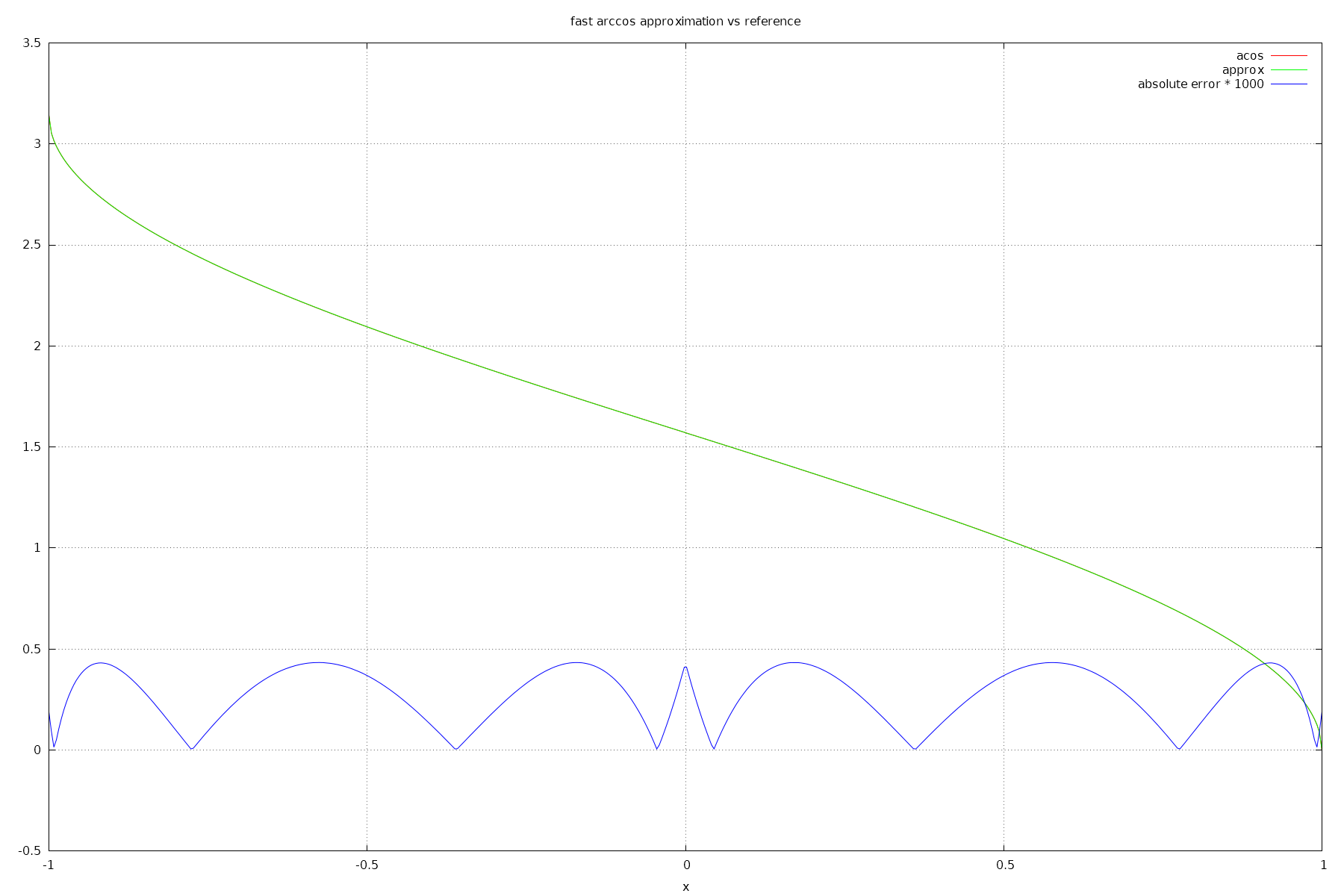
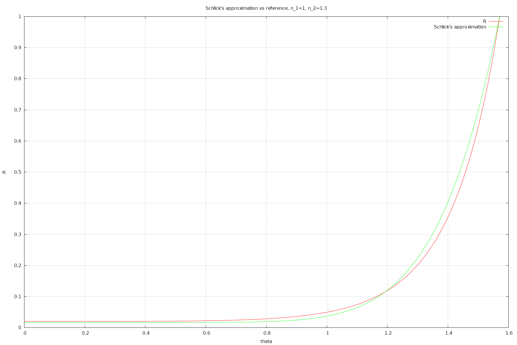
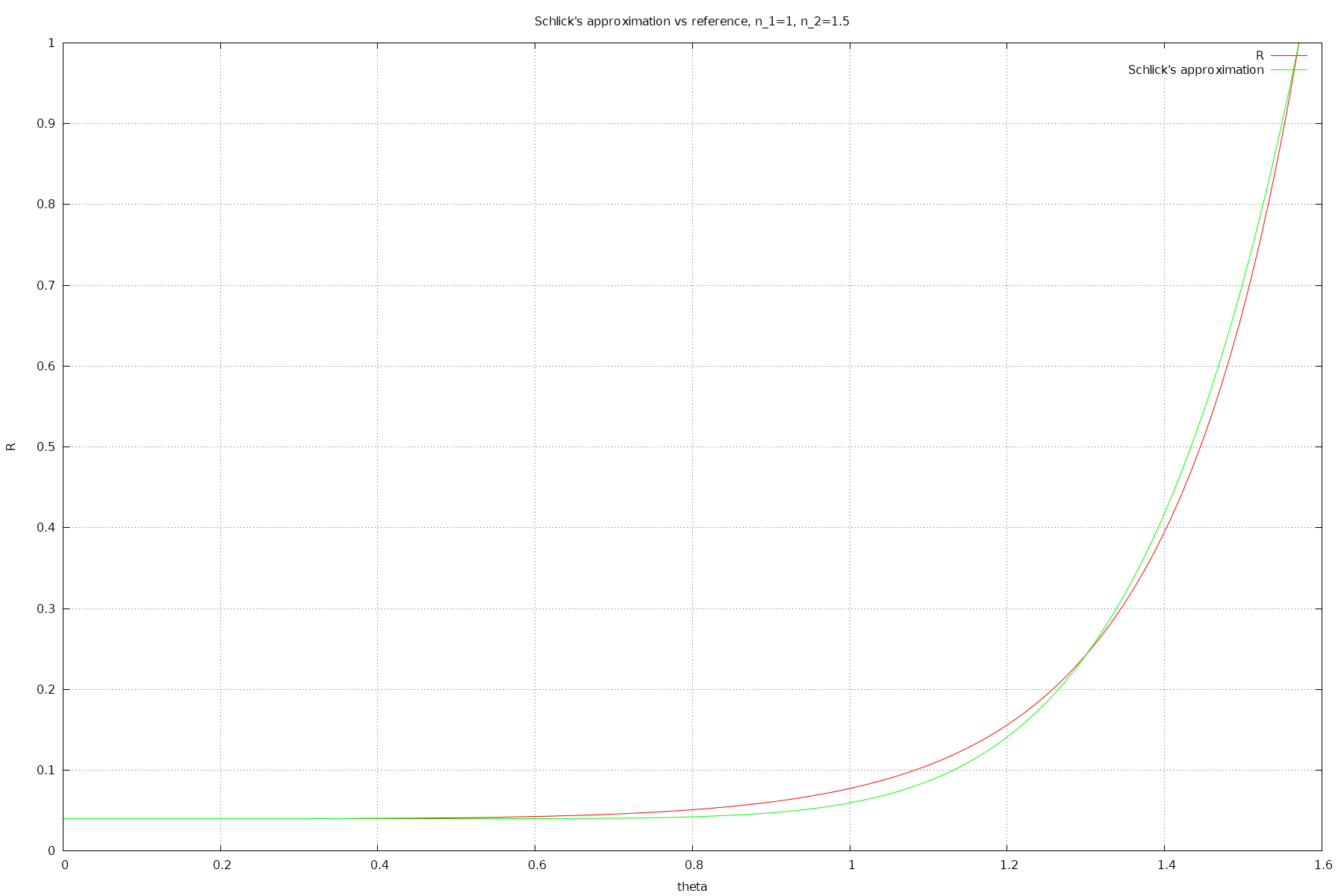
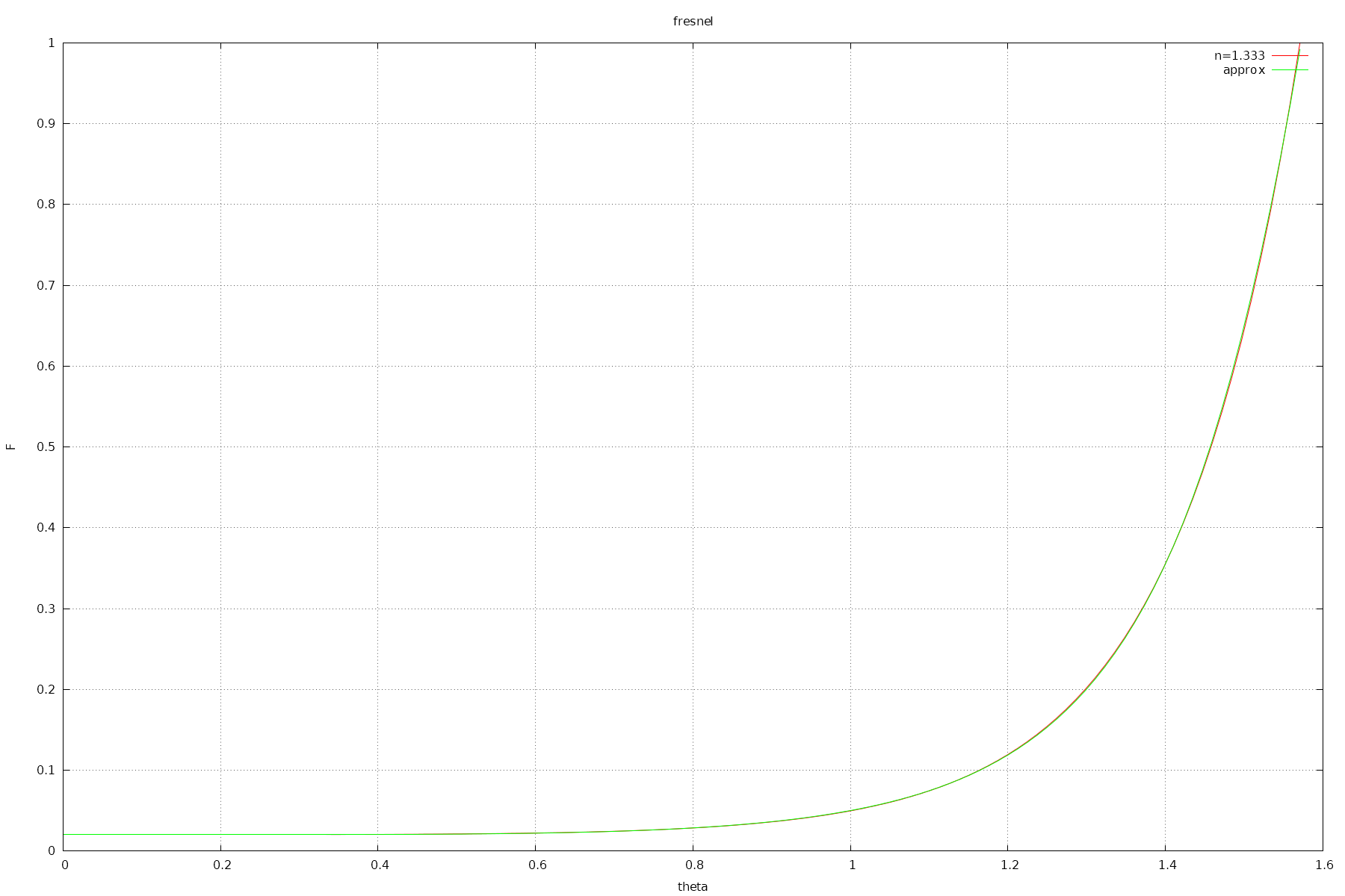
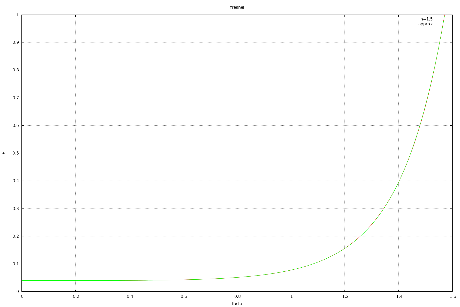
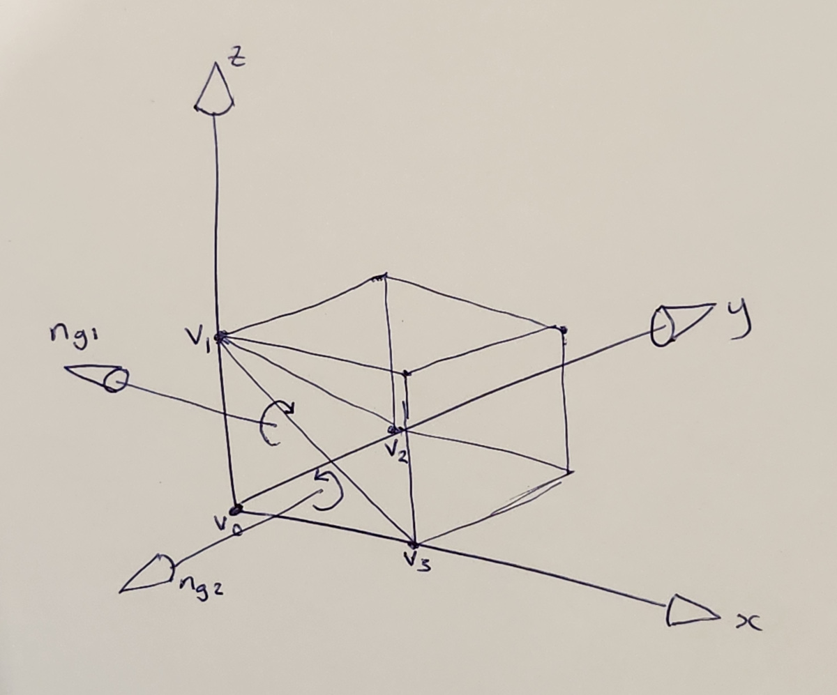 The unit cube, with geometric normals
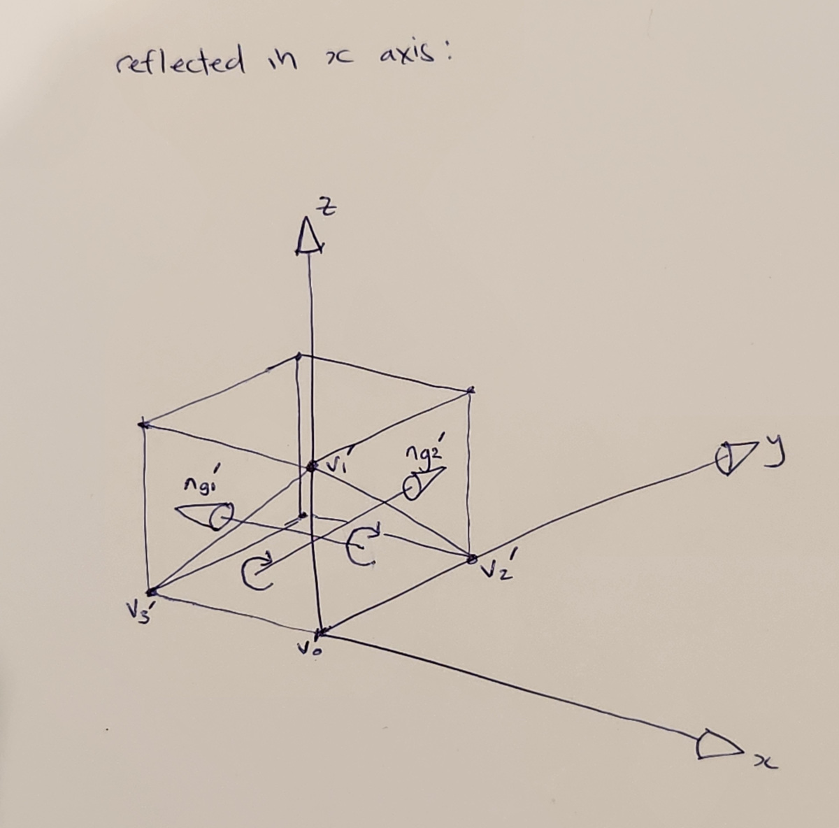 The unit cube reflected along the x-axis, with resulting geometric normals
 Adjugate transpose used, no reflection transformation
 sign(det) x Adjugate transpose used (similar to inverse transpose), no reflection transformation
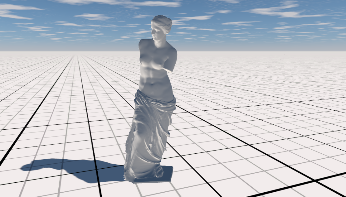 Adjugate transpose used, with reflection transformation - incorrect rendering
 sign(det) x Adjugate transpose used (similar to inverse transpose), with reflection transformation - correct rendering
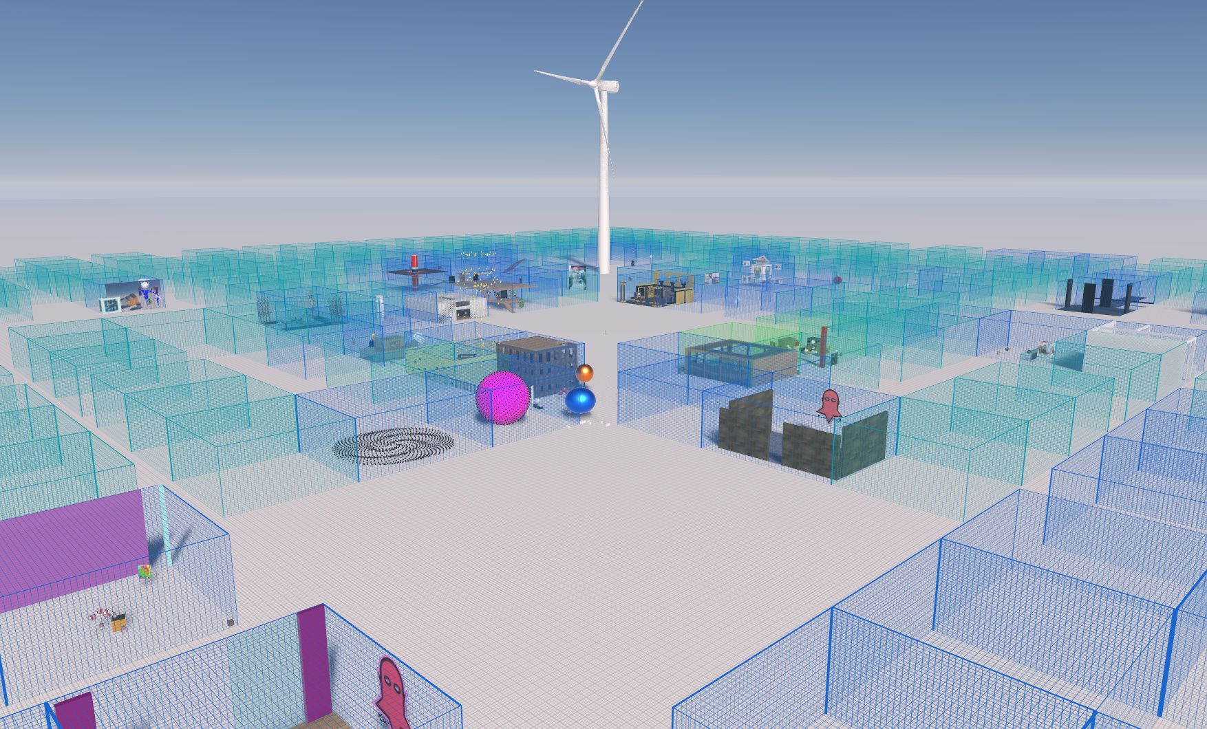


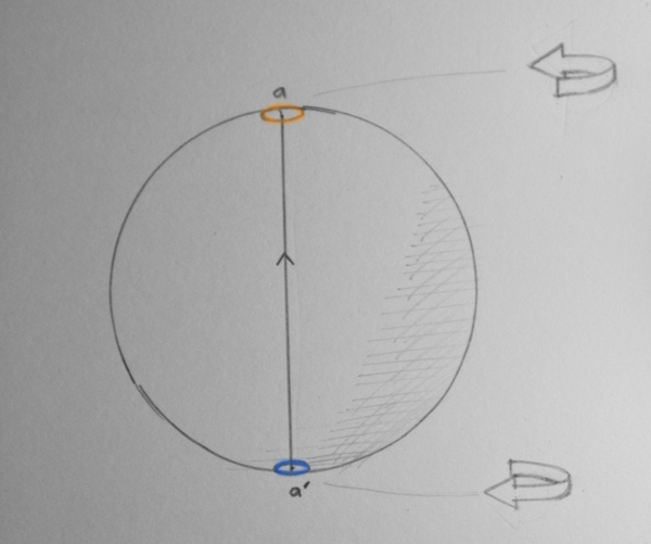 A path from \(-\pi\) to \(\pi\) rotation

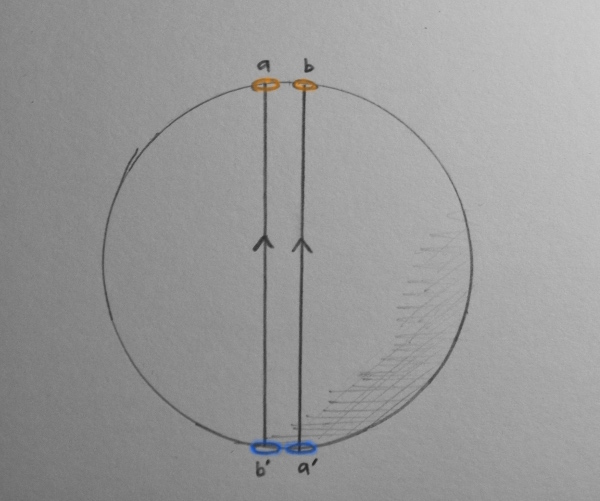 A path from \(-2\pi\) to \(2pi\) rotation. Note that the path enters portal a and exits portal a', then enters portal b and then exits portal b'. The paths are shown slightly separated for clarity.

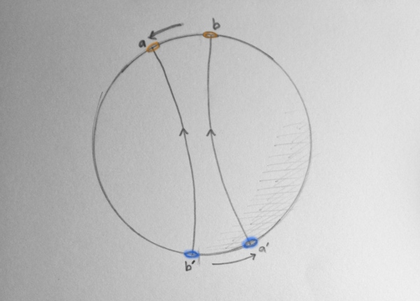 A deformation of a \(4\pi\) rotation.
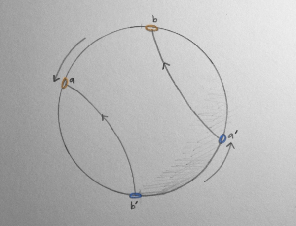 A deformation of a \(4\pi\) rotation.
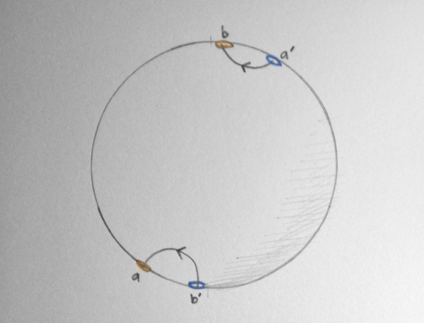 A deformation of a \(4\pi\) rotation.
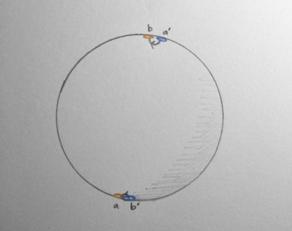 A deformation of a \(4\pi\) rotation.